Box Plot. Customarily, a batch of data is summarized by its average
and standard deviation. These two numerical values characterize a nor-
mal distribution, as explained in expression (2- 0). Certain features of the
data, e.g. , skewness and extreme values , are not reflected in the average and
standard deviation. The box plot (due also to Tukey) presents graphically
a five-number summary which, in many ca.ses, shows .more of the original
features of the batch of data then the two number summary.
To construct a box plot , the sample of numbers are first ordered from
the smallest to the largest , resulting in
(I), (2),... (n)'
U sing a set of rules , the median, m, the lower fourth Ft., and the upper
fourth Fu, are calculated. By definition, the int~rval (Fu - Ft.) contains half
of all data points. We note that m u, and Ft. are not disturbed by outliers.
The interval (Fu Ft.) is called the fourth spread. The lower cutoff limit
Ft. 1.5(Fu Ft.)
and the upper cutoff limit is
Fu 1.5(F Ft.).
A "box" is then constructed between Pt. and u, with the median line
dividing the box into two parts. Two tails from the ends of the box extend
to Z (I) and Z en) respectively. If the tails exceed the cutoff limits , the cutoff
limits are also marked.
From a box plot one can see certain prominent features of a batch of
data:
1. Location - the median, and whether it is in the middle of the box.
2. Spread - The fourth spread (50 percent of data): - lower and upper
cut off limits (99. 3 percent of the data will be in the interval if the
distribution is normal and the data set is large).
3. Symmetry/skewness - equal or different tail lengths.
4. Outlying data points - suspected outliers.
Simpo PDF Merge and Split Unregistered Version - http://www.simpopdf.com
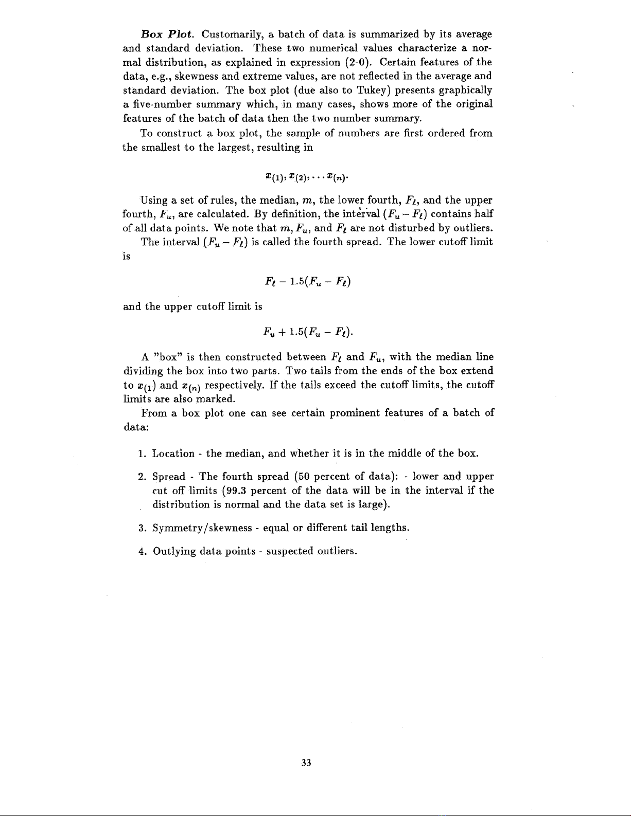
The 48 measurements of isotopic ratio bromine (79/81) shown in Fig. 1
were actually made on two instruments, with 24 measurements each. Box
plots for instrument instrument II, and for both instruments ate shown in
Fig. 2.
310
300
290
280
270
260
X(N), LARGEST
UPPER FOURTH
MEDIAN
, '
LOWER FOURTH
--
LOWER CUTOFF LIMIT
X(I), SMALLEST
INSTRUMENT I INSTRUMENT II COMBINED I & II
FIg. 2. Box plot of isotopic ratio, bromine (79/91).
X(1)
The five numbersumroary for the 48 data point is , for the combined data:
Smallest:
Median
Lower Fourth Xl:
Upper Follrth
Largest: (n)
261
(n + 1)/2 = (48 + 1)/2 = 24.
(m) if m is an integer;
(M) + Z (M+l))/2 if not;
where is the largest integer
not exceeding m.
(291 + 292)/2 = 291.5
(M + 1)/2 = (24 + 1)/2 = 12.
(i) if is an integer;
(L) = z(L + 1))/2 if not,
where is the largest integer
not exceeding
(284 + 285)/2 = 284.
+ 1 - = 49 ~ 12.5 = 36.
(u) if is an integer;
(U) + z(U+l)J/2 ifnot,
where is the largest integer
not exceeding
(296 + 296)/2 = 296
305
Simpo PDF Merge and Split Unregistered Version - http://www.simpopdf.com
Box plots for instruments I and II are similarly constructed. It seems
apparent from these two plots that (a) there was a difference between the
results for these two instruments, and (b) the precision of instrument II is
better than that of instrument I. The lowest value of instrument I, 261 , is
less than the lower cutoff for the plot of the combined data, but it does not
fall below the lower cutoff for instrument I alone. As an exercise, think of
why this is the case.
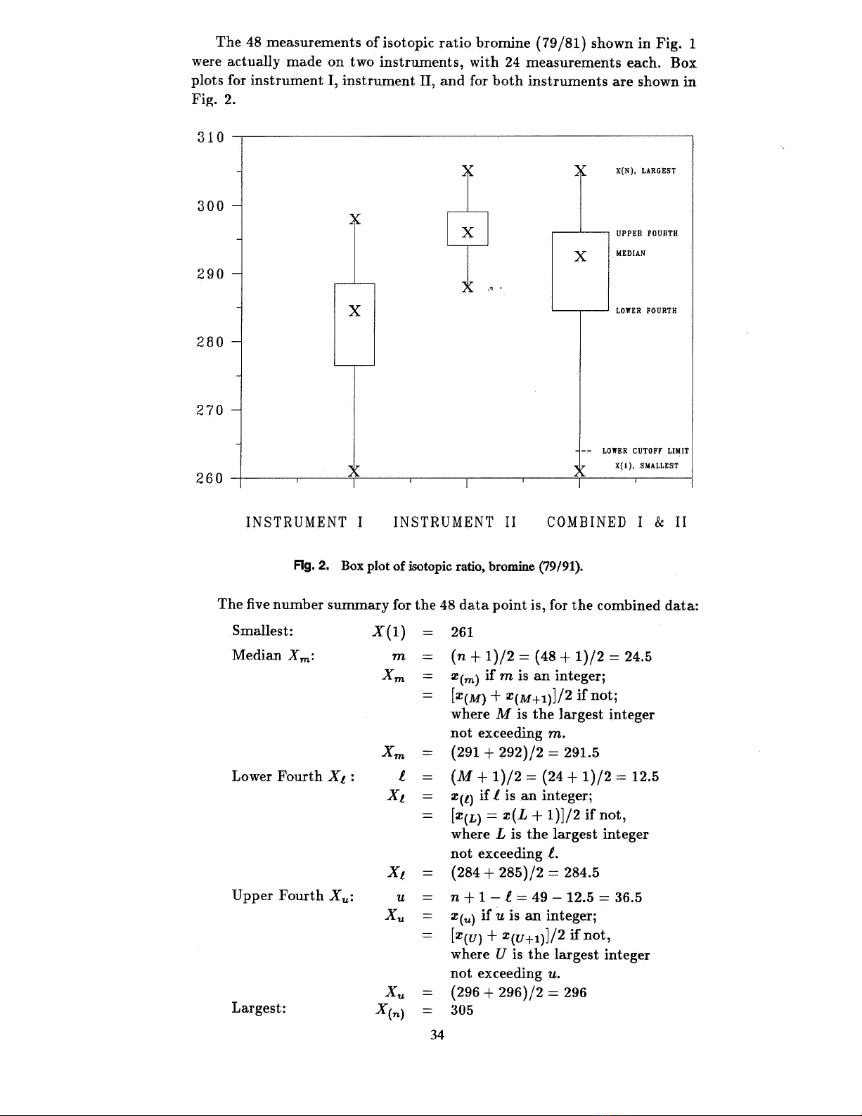
Box plots can be used to compare several batches of data .effectively
and easily. Fig. 3 is a box plot of the amount of magnesium in different
parts of a long alloy rod. The specimen number represents the distance, in
meters , from the edge of the 100 meter rod to the place where the specimen
was taken. Ten determinations were made at the selected locations for each
specimen. One outlier appears obvious; there'is also a mild indication of
decreasing content of magnesium along the rod. -
Variations of box plots are giyen in 13) and (4).
C":J
E-'
I:J:::
0...
E-'
;:g;:::.'-';:g
CUTOFF
X(N) LARGEST
UPPER FOURTH
MEDI N
LOWE FOURTH
X( 1) SMALLEST
BARl BAR5 BAR20 BAR50 BAR85
FIg. 3. Magnesium content of specimens taken.
Plots for Checking on Models and Assumptions
In making measurements , we may consider that each measurement is
made up of two parts , one fixed and one variable, Le.
Measurement = fixed part + variable part
, in other words
Data = model + error.
We use measured data to estimate the fixed part , (the Mean, for ex-
ample), and use the variable part (perhapssununarized by the standard
deviation) to assess the goodness of our estimate.
Simpo PDF Merge and Split Unregistered Version - http://www.simpopdf.com
Residuals. Let the ith data point be denoted by Yi, let the fixed part
be a constant and let the random error be (;i as used in equation (2- 19).
Then
Yi (;i, i=1,
,...
IT we use the method of least squares to estimate m, the resulting esti-
mate is
m=y= LyiJn
or the average of all measurements.
The ith residual Ti, is defined as the difference between the ith data
point and the fitted constant, Le.
' '
Ti Yi
In general , the fixed part can be a function of another variable (or
more than one variable). Then the model is
Yi (zd + (;i
and the ith residual is defined as
Ti Yi F(zd,
where F( Zi) is the value ofthe function computed with the fitted parameters.
IT the relationship between and is linear as in (2- 21), then Ti Yi
(a bzd where and are the intercept and the slope of the fitted straight
line, respectively.
When, as in calibration work, the values of F(Zi) are frequently consid-
ered to be known, the differences between measured values and known values
will be denoted di, the i th deviation , and can be used for plots instead of
residuals.
Adequacy of Model. Following is a discussion of some of the issues
involved in checking the adequacy of models and assumptions. For each
issue, pertinent graphical techniques involving residuals or deviations are
presented.
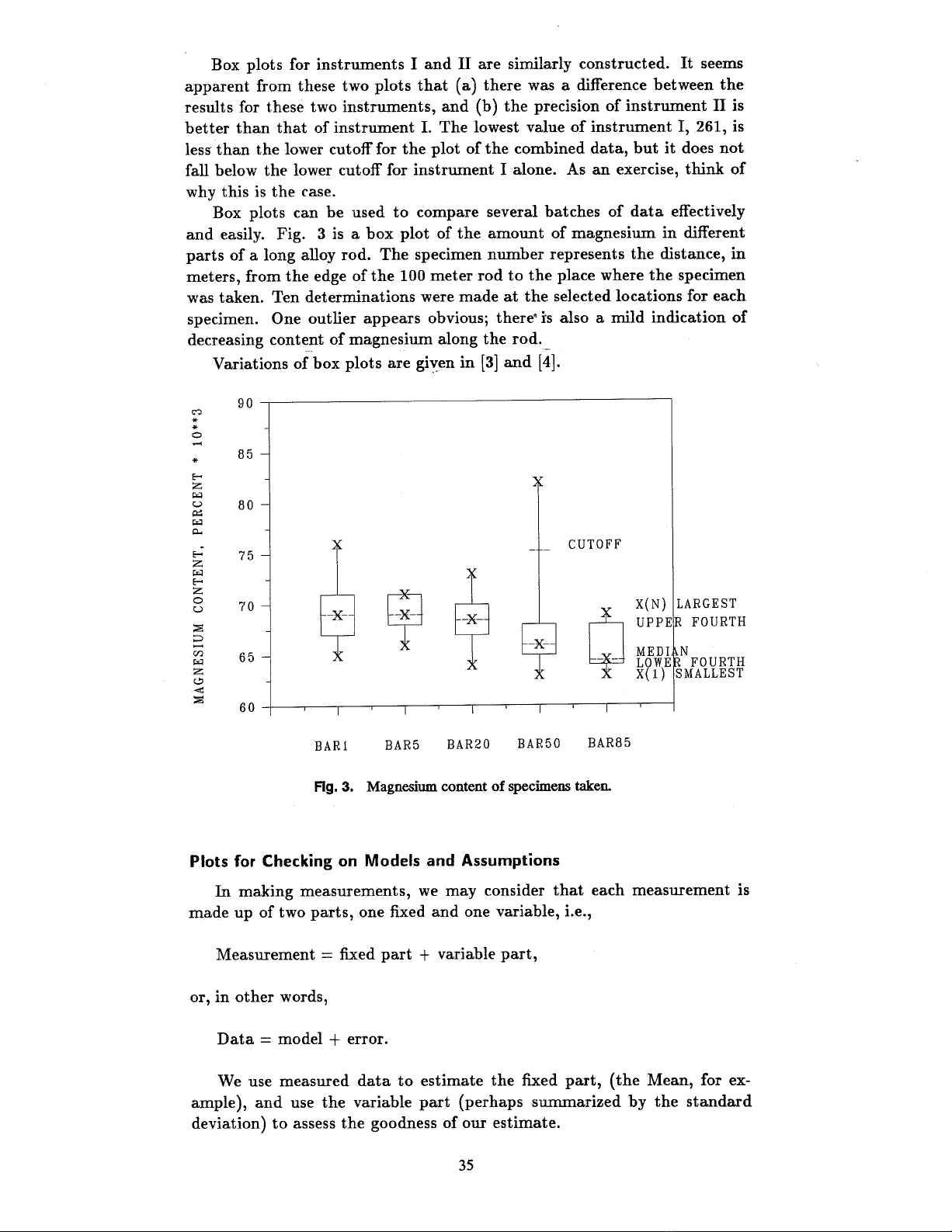
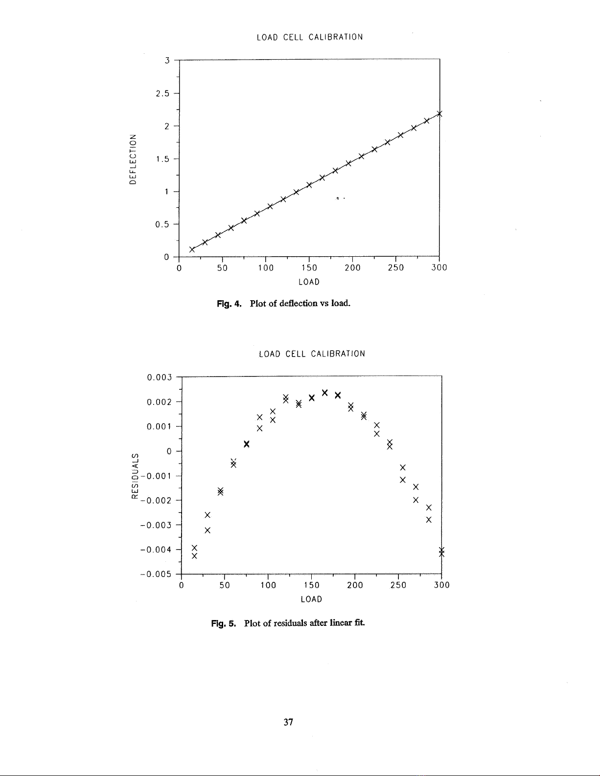
In calibrating a load cell, known deadweights are added in sequence and
the deflf:'ctions are read after each additional load. The deflections are plot-
ted against Joads in Fig. 4. A straight line model looks plausible , Le.
(deflection d = bI (loadd.
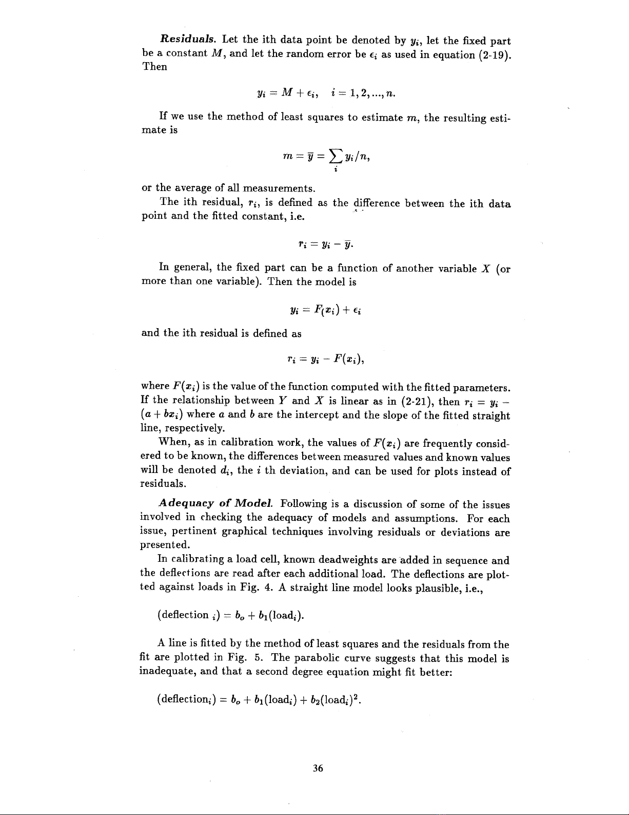
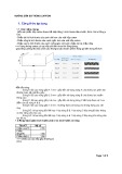
A line is fitted by the method of least squares and the residuals from the
fit are plotted in Fig. 5. The parabolic curve suggests that this model is
inadequate, and that a second degree equation might fit better:
(deflectiond = bI (loadi) + b2(loadd2
Simpo PDF Merge and Split Unregistered Version - http://www.simpopdf.com
f--,-
1.5
'-'-
003
002
001
(I)
0:(
;S~ 001 ~
(/)
0:: ~ O02 ~
003 -
004 -
~0. 005
LOAD CELL CALIBRATION
100 200 300150
LOAD
250
Ag. 4. Plot of deflection vS load.
LOAD CELL CALIBRATION
X X X
X ~
250
150
LOAD
200
100 300
Fig. 5. Plot of residuals after linear fit.
Simpo PDF Merge and Split Unregistered Version - http://www.simpopdf.com
![Bảng tra dung sai lắp ghép Lê Hoàng Lâm: [Thêm từ mô tả phù hợp]](https://cdn.tailieu.vn/images/document/thumbnail/2022/20221205/camtucau205/135x160/9731670233749.jpg)


![Cẩm nang Gia công kim loại Việt Nam [mới nhất]](https://cdn.tailieu.vn/images/document/thumbnail/2026/20260513/baobinh_011/135x160/7971778670576.jpg)


![Giáo trình Hàn ống nâng cao (Nghề Hàn - CĐ) Trường Cao đẳng nghề Hải Dương [Mới nhất]](https://cdn.tailieu.vn/images/document/thumbnail/2025/20251212/laphong0906/135x160/47521779076565.jpg)


%20--%3e%3cdefs%3e%3cstyle%3e%20.st0%20{%20fill:%20%23fff;%20}%20.st1%20{%20fill:%20%237800fa;%20}%20%3c/style%3e%3c/defs%3e%3cpath%20class='st1'%20d='M117.78,12.18H43.11c2.9,3.47,4.65,7.94,4.65,12.82,0,5.6-2.3,10.66-6.01,14.29h76.02l7.22-13.56-7.22-13.56Z'/%3e%3cg%3e%3cpath%20class='st0'%20d='M53.58,26.17h-.59v-1.46h.59v-4.96h2.83c1.78,0,2.67.94,2.67,2.82v5.76c0,1.87-.89,2.81-2.67,2.81h-2.83v-4.96ZM55.36,21.37v3.34h1.1v1.46h-1.1v3.34h1.01c.61,0,.91-.37.91-1.1v-5.93c0-.74-.3-1.1-.91-1.1h-1.01Z'/%3e%3cpath%20class='st0'%20d='M65.99,31.14h-1.8l-.31-2.07h-2.19l-.31,2.07h-1.64l1.82-11.39h2.62l1.82,11.39ZM65.28,18.04c-.25.46-.51.77-.75.94-.21.15-.47.22-.79.22-.26,0-.57-.07-.92-.22l-.38-.15c-.14-.05-.26-.07-.37-.07-.3,0-.53.18-.71.54l-.91-.68c.25-.46.51-.77.75-.94.21-.14.48-.21.79-.21.26,0,.57.07.92.21l.38.15c.14.05.26.07.37.07.3,0,.53-.18.71-.54l.91.68ZM61.91,27.52h1.73l-.87-5.76-.87,5.76Z'/%3e%3cpath%20class='st0'%20d='M74.53,26.89v1.52c0,1.91-.89,2.86-2.67,2.86s-2.67-.95-2.67-2.86v-5.93c0-1.91.89-2.86,2.67-2.86s2.67.95,2.67,2.86v1.11h-1.69v-1.22c0-.75-.31-1.12-.93-1.12s-.93.37-.93,1.12v6.15c0,.74.31,1.11.93,1.11s.93-.37.93-1.11v-1.63h1.69Z'/%3e%3cpath%20class='st0'%20d='M81.4,31.14h-1.8l-.31-2.07h-2.19l-.31,2.07h-1.64l1.82-11.39h2.62l1.82,11.39ZM75.9,19.2l1.52-1.91h1.71l1.51,1.91h-1.61l-.76-.95-.75.95h-1.61ZM77.32,27.52h1.73l-.87-5.76-.87,5.76ZM83.1,15.99l-1.76,1.91h-1.26l1.17-1.91h1.86Z'/%3e%3cpath%20class='st0'%20d='M84.86,19.75c1.78,0,2.67.94,2.67,2.82v1.48c0,1.87-.89,2.81-2.67,2.81h-.85v4.28h-1.79v-11.39h2.64ZM84.01,21.37v3.86h.85c.58,0,.87-.36.87-1.08v-1.71c0-.71-.29-1.07-.87-1.07h-.85Z'/%3e%3cpath%20class='st0'%20d='M93.51,19.75c1.78,0,2.67.94,2.67,2.82v1.48c0,1.87-.89,2.81-2.67,2.81h-.85v4.28h-1.79v-11.39h2.64ZM92.66,21.37v3.86h.85c.58,0,.87-.36.87-1.08v-1.71c0-.71-.29-1.07-.87-1.07h-.85Z'/%3e%3cpath%20class='st0'%20d='M98.8,31.14h-1.79v-11.39h1.79v4.88h2.03v-4.88h1.83v11.39h-1.83v-4.88h-2.03v4.88Z'/%3e%3cpath%20class='st0'%20d='M105.36,24.55h2.46v1.62h-2.46v3.34h3.09v1.63h-4.88v-11.39h4.88v1.63h-3.09v3.18ZM108.17,17.29l-1.76,1.91h-1.26l1.17-1.91h1.86Z'/%3e%3cpath%20class='st0'%20d='M112.2,19.75c1.78,0,2.67.94,2.67,2.82v1.48c0,1.87-.89,2.81-2.67,2.81h-.85v4.28h-1.79v-11.39h2.64ZM111.35,21.37v3.86h.85c.58,0,.87-.36.87-1.08v-1.71c0-.71-.29-1.07-.87-1.07h-.85Z'/%3e%3c/g%3e%3ccircle%20class='st1'%20cx='25'%20cy='25'%20r='20'/%3e%3cpath%20class='st0'%20d='M32.78,19.27c2.92,0,4.43,2.55,5.28,5.33l.71,2.17c.14.38-.33.75-.71.75h-5.61c.19-.33.24-.71.09-1.08l-.75-2.45c-.43-1.32-.99-2.64-1.79-3.77.75-.57,1.65-.94,2.78-.94h0ZM25,18.38c3.25,0,4.9,2.78,5.89,5.89l.76,2.45c.14.42-.33.8-.8.8h-11.69c-.42,0-.94-.38-.8-.8l.75-2.45c.99-3.11,2.64-5.89,5.89-5.89h0ZM25,11.35c1.74,0,3.11,1.37,3.11,3.11s-1.37,3.11-3.11,3.11-3.11-1.41-3.11-3.11,1.41-3.11,3.11-3.11h0ZM17.27,19.27c1.08,0,1.98.38,2.73.94-.8,1.13-1.37,2.45-1.74,3.77l-.8,2.45c-.14.38-.05.75.09,1.08h-5.56c-.42,0-.9-.38-.75-.75l.71-2.17c.9-2.78,2.41-5.33,5.33-5.33h0ZM17.27,12.91c1.51,0,2.78,1.27,2.78,2.83s-1.27,2.83-2.78,2.83-2.83-1.27-2.83-2.83,1.27-2.83,2.83-2.83h0ZM32.78,12.91c1.56,0,2.78,1.27,2.78,2.83s-1.23,2.83-2.78,2.83-2.83-1.27-2.83-2.83,1.27-2.83,2.83-2.83h0ZM27.07,28.56v.09c0,.57-.24,1.08-.61,1.46h0v.05c-.38.33-.9.57-1.46.57s-1.08-.24-1.46-.61h0c-.38-.38-.61-.9-.61-1.46v-.09h1.41v.09c0,.19.05.38.19.47v.05c.09.09.28.19.47.19s.38-.09.47-.19v-.05c.14-.09.24-.28.24-.47t-.05-.09h1.41ZM30.99,28.56v.09c0,1.65-.66,3.16-1.74,4.24-1.08,1.08-2.59,1.79-4.24,1.79s-3.16-.71-4.24-1.79l-.05-.05c-1.04-1.08-1.7-2.55-1.7-4.2v-.09h1.41v.09c0,1.27.47,2.4,1.27,3.25h.05c.85.85,1.98,1.37,3.25,1.37s2.4-.52,3.25-1.37c.85-.8,1.37-1.98,1.37-3.25v-.09h1.37ZM34.99,28.56v.09c0,2.78-1.13,5.28-2.92,7.07-1.79,1.79-4.29,2.92-7.07,2.92s-5.23-1.13-7.07-2.92c-1.79-1.79-2.92-4.29-2.92-7.07v-.09h1.41v.09c0,2.4.94,4.53,2.5,6.08,1.56,1.56,3.72,2.5,6.08,2.5s4.52-.94,6.08-2.5c1.56-1.56,2.5-3.68,2.5-6.08v-.09h1.41Z'/%3e%3c/svg%3e)