Linear
versus
nonlinear
methods
of
sire
evaluation
for
categorical
traits :
a
simulation
study
A.
MEIJERING
D.
GIANOLA
*
Department
of
Animal
Science,
University
of
Illinois,
Urbana,
Illinois
61801,
U.S.A.
**
On
leave
from :
Research
Institute
for
Animal
Production
«
Schoonoord
»
3700
AM
Zeist,
The
Netherlands
Summary
Linear
(BLUP)
and
nonlinear
(GFCAT)
methods
of
sire
evaluation
for
categorical
data
were
compared
using
Monte
Carlo
techniques.
Binary
and
ordered
tetrachotomous
responses
were
generated
from
an
underlying
normal
distribution
via
fixed
thresholds,
so
as
to
model
incidences
in
the
population
as
a
whole.
Sires
were
sampled
from
a
normal
distribution
and
family
structure
consisted
of
half-sib
groups
of
equal
or
unequal
size ;
simulations
were
done
at
several
levels
of
heritability
(h2).
When
a
one-way
model
was
tenable
or
when
responses
were
tetrachotomous,
the
differences
between
the
2
methods
were
negligible.
However,
when
responses
were
binary,
the
layout
was
highly
unbalanced
and
a
mixed
model
was
appropriate
to
describe
the
underlying
variate,
GFCAT
elicited
significantly
larger
responses
to
truncation
selection
than
BLUP
at
h2
=
.20
or
.50
and
when
the
incidence
in
the
population
was
below
25
p.
100.
The
largest
observed
difference
in
selection
efficiency
between
the
2
methods
was
12
p.
100.
Key
words :
Categorical
data,
sire
evaluation,
threshold
traits,
nonlinear
models,
simulation.
Résumé
Méthodes
linéaires
et
non
linéaires
d’évaluation
des
pères
sur
des
caractères
discrets :
étude
par
simulation
Des
méthodes
linéaires
(BLUP)
et
non
linéaires
(GFCAT)
d’évaluation
des
pères
sur
données
discrètes
ont
été
comparées
à
l’aide
des
techniques
de
Monte
Carlo.
On
a
simulé
des
réponses
selon
2
ou
4
catégories
à
partir
d’une
distribution
normale
sous-jacente
munie
de
seuils
fixés.
Les
pères
ont
été
échantillonnés
dans
une
distribution
normale.
La
structure
famille
comportait
des
groupes
de
demi-germains
de
taille
égale
ou
inégale.
Les
simulations
ont
été
effectuées
pour
plusieurs
niveaux
d’héritabilité
(h
2
).
Les
différences
entre
les
2
méthodes
d’évaluation
sont
négligeables
avec
un
modèle
à y
une
voie
ou
des
réponses
en
4
classes.
Toutefois,
en
présence
de
réponses
binaires,
d’un
dispositif
fortement
déséquilibré
et
d’une
sous-jacente
décrite
en
modèle
mixte,
la
procédure
GFCAT
procure
des
réponses
après
sélection
par
troncature
significativement
supérieures
à
celles
obtenues
avec
le
BLUP
pour
h2
=
0,20
et
0,50
et
une
incidence
du
caractère
dans
la
population
inférieure
à
25
p.
100.
La
di
y
fférence
maximum
d’efficacité
de
sélection
observée
entre
ces
deux
méthodes
s’est
située
à
12
p.
100.
Mots
clés :
Données
discrètes,
évaluation
des
pères,
caractères
à
seuils,
modèle
non
linéaire,
simulation.
I.
Introduction
Prediction of
genetic
merit
of
individuals
from
observations
on
relatives
is
of
basic
importance
in
animal
breeding.
If
the
records
and
the
genetic
values
to
be
predicted
follow
a
joint
normal
distribution,
best
linear
unbiased
prediction
(BLUP)
is
the
method
of
choice,
because
it
yields
the
maximum
likelihood
estimator of
the
best
predictor,
it
maximizes
the
probability
of
correct
pairwise
ranking
(H
ENDERSON
,
1973)
and
more
relevantly,
it
maximizes
genetic
progress
among
translation
invariant
rules
when
selecting
a
fixed
number
of
candidates
(G
OFFINET
,
1983 ;
F
ERNANDO
,
1983).
However,
a
number
of
traits
of
importance
in
animal
production
(e.g.,
calving
ease,
livability,
disease
suscep-
tibility,
type
scores)
are
measured
as
a
response
in
a
small
number
of
mutually
exclusive,
exhaustive
and
usually
ordered
categories.
These
variates
are
not
normally
distributed
and,
in
this
case,
linear
predictors
may
behave
poorly
for
ranking
purposes
(P
ORTNOY
,
1982).
G
IANOLA
(1980,
1982)
discussed
additional
potential
drawbacks
of
linear
predictors
for
sire
evaluation
with
categorical
data,
arguing
from
the
viewpoint
of
«
threshold
»
models
for
meristic
traits
(D
EMPSTER
&
L
ERNER
,
1950 ;
FALCONER,
1981).
S
CHAEFFER
&
W
ILTON
(1976)
examined
a
modified
version
of
a
(fixed)
linear
model
for
analysis
of
categorical
data
developed
by
GRIZZLE
et
al.
(1969).
They
suggested
that
the
use
of
BLUP
methodology
in
sire
evaluation
for
categorical
responses
might
be
justified
given
certain
sampling
conditions
which
unfortunately
are
inconsistent
with
the
assumptions
required
by
their
model.
This
work
gave
impetus
for
widespread
use
of
BLUP
in
evaluation
of
sires
for
categorical
variates
(e.g.,
B
ERGER
&
FREEMAN,
1978 ;
V
AN
V
LECK
&
K
ARNER
,
1979 ;
C
ADY
&
B
URNSIDE
,
1982 ;
W
ESTELL
et
C
ll.,
1982).
G
IANOLA
&
F
OULLEY
(1983a)
developed
a
Bayesian
nonlinear
method
of
sire
eva-
luation
for
categorical
variates
based
on
the
«
threshold
concept.
In
this
approach
(GFCAT
=
Gianola-Foulley-Categorical),
the
probability
of
response
in
a
given
category
is
assumed
to
follow
a
normal
integral
with
an
argument
dependent
on
fixed
thresholds
and
on
a
location
parameter
in
a
conceptual
underlying
distribution.
The
location
parameter
is
modeled
as
a
linear
combination
of
fixed
effects
and
random
variables.
Prior
information
on
the
distribution
of
the
parameters
of
the
model
is
combined
with
the
likelihood
of
the
data
to
yield
a
posterior
density
function,
the
mode
of
which
is
then
taken
as
an
approximation
to
the
posterior
mean
or
optimum
ranking
rule
in
the
sense
of
COC
HRAN
(1951),
BULMER
(1980),
F
ERNANDO
(1983)
&
GO
FFINET
(1983).
Solution
of
the
resulting
equations
requires
an
iterative
implementation.
A
conceptually
similar
method
has
been
developed
by
H
ARVILLE
&
M
EE
(1982).
Although
these
pro-
cedures
are
theoretically
appealing,
computations
are
more
complicated
than
those
arising
in
linear
methodology.
Although
BLUP
has
become
a
standard
method
of
sire
evaluation
in
many
countries,
its
robustness
to
departures
from
linearity
has
not
been
examined.
Non
linearity
arises
with
categorical
data
and,
therefore,
a
comparison
between
BLUP
and
the
procedure
developed
by
G
IANOLA
&
F
OULLEY
(1983
a)
is
of
interest.
The
objective
of
this
paper
is
to
present
results
of
a
Monte
Carlo
comparison
of
the
ability
of
the
above
2
methods
to
rank
sires
correctly
when
applied
to
simulated
categorical
data.
II.
Methodology
A.
Experimental
design
and
simulation
of
data
Three
experimental
settings
were
considered
to
compare
the
2
methods
of
evalua-
tion :
1)
a
one-way
sire
model
with
equal
progeny
group
size
within
a
data
set ;
2)
a
one-way
sire
model
with
unequal
progeny
group
size
within
a
data
set ;
and
3)
a
mixed
model
with
unequal
group
size
within
a
data
set.
In
the
1st
setting
36
independent
data
sets
were
generated
per
replicate.
These
data
sets
represented
all
combinations
of
3
progeny
group
sizes
(10,
50
or
250
progeny
records
for
each
of
50
sires),
3
levels
of
heritability
in
a
conceptual
underlying
scale
(h
z
=
0.05,
0.20
or
0.50),
and
4
types
of
categorization
which
will
be
described
later.
Phenotypic
values
in
the
underlying
scale
were
generated
(RO
NNINGEN
,
1974 ;
O
LAUSSON
&
RO
NNINGEN
,
1975)
as :
where :
Yij
:
phenotype
of
individual j
in
progeny
group
i,
with
y, -
N
(0,1) ;
h2:
heritability
in
the
underlying
scale ;
a;
:
standard
normal
random
variate
common
to
all
individuals
in
progeny
group
i
with
ai
-
N
(0,1),
and
a
ij :
standard
normal
random
variate
for
individual j
in
progeny
group
i,
with
a,
rv
N
(0,1).
The
phenotypes
y;!
were
categorized
using
fixed
thresholds
in
the
standard
normal
distribution
function.
The
first
3
categorizations
reflected either
a 1 p.
100
(y;!
>
2.33),
5
p.
100
(y,
>
1.65)
or
25
p.
100
(y;!
>
0.68)
incidence
of
a
binary
trait
in
the
population
as
a
whole.
The
4,h
type
of
categorization
created
a
tetrachotomous
trait
reflecting
incidences
of
40
p.
100-40
p.
100-15
p.
100-5
p.
100
in
the
population
as a
whole ;
this
was
made
using
3
thresholds
(yij
:=:; - .25 ; -
.25 <
yq
:=:;
.84 ;
.84
<
y,
<-
1.65 ;
yq
>
1.65).
Binary
responses
were
coded
as
0-1,
and
tetrachotomies
were
coded
using
the
integer
values
1
to
4.
The
difference
in
heritability
in
a
categorical
scale
resulting
from
using
integer
verus
«
optimal
»
scores
is
negligible
(G
IANOLA
&
NoRTOrt,
1981).
In
the
2n
d
setting
12
independent
data
sets
were
generated
per
replicate,
representing
all
combinations
of the
above
levels
of
heritability
and
categorization.
However,
the
50
progeny
groups
represented
in
each
data
set
varied
between
5
and
250
in
steps
of
5.
Data
were
simulated
as
outlined
for
Setting
1.
In
Setting
3,
15
independent
data
sets
were
generated
per
replicate.
Combinations
of
the
3
heritability
levels
with
a
10
p.
100
incidence
level
(y;!
>
1.28)
of
a
binary
trait
were
added
to
those
used
in
Setting
2.
Data
were
generated
as
before.
Prior
to
catego-
rization,
the
effects
of
2
fixed
classifications,
factor
A
(2
levels)
and
factor
B
(10
levels),
were
superimposed,
as
indicated
in
table
1.
Each
progeny
group
was
almost
equally
represented
in
the
levels
of
factor
A,
but
only
in
2
levels
of
factor
B
(20
p.
100
in
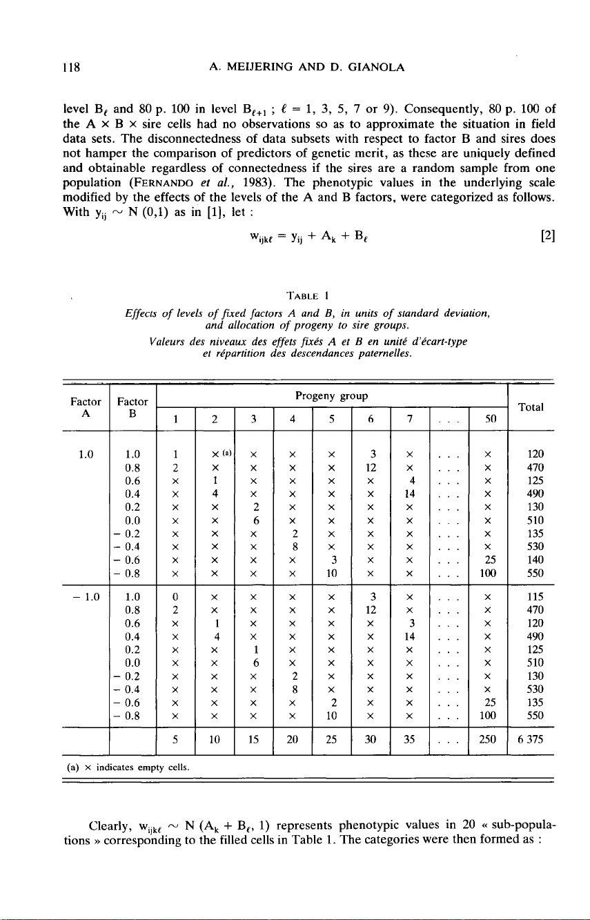
level
B,
and
80
p.
100
in
level
Be+, ;
e =
1,
3,
5,
7
or
9).
Consequently,
80
p.
100
of
the
A
x
B
x
sire
cells
had
no
observations
so
as
to
approximate
the
situation
in field
data
sets.
The
disconnectedness
of
data
subsets
with
respect
to
factor
B
and
sires
does
not
hamper
the
comparison
of
predictors
of
genetic
merit,
as
these
are
uniquely
defined
and
obtainable
regardless
of
connectedness
if
the
sires
are
a
random
sample
from
one
population
(F
ERNANDO
et
al.,
1983).
The
phenotypic
values
in
the
underlying
scale
modified
by
the
effects
of
the
levels
of
the
A
and
B
factors,
were
categorized
as
follows.
With
y,
j
-
N
(0,1)
as
in
[1],
let :
Clearly,
Wijkf
rv
N
(A
k
+
B!,
1)
represents
phenotypic
values
in
20
«
sub-popula-
tions
»
corresponding
to
the
filled
cells
in
Table
1.
The
categories
were
then
formed
as :
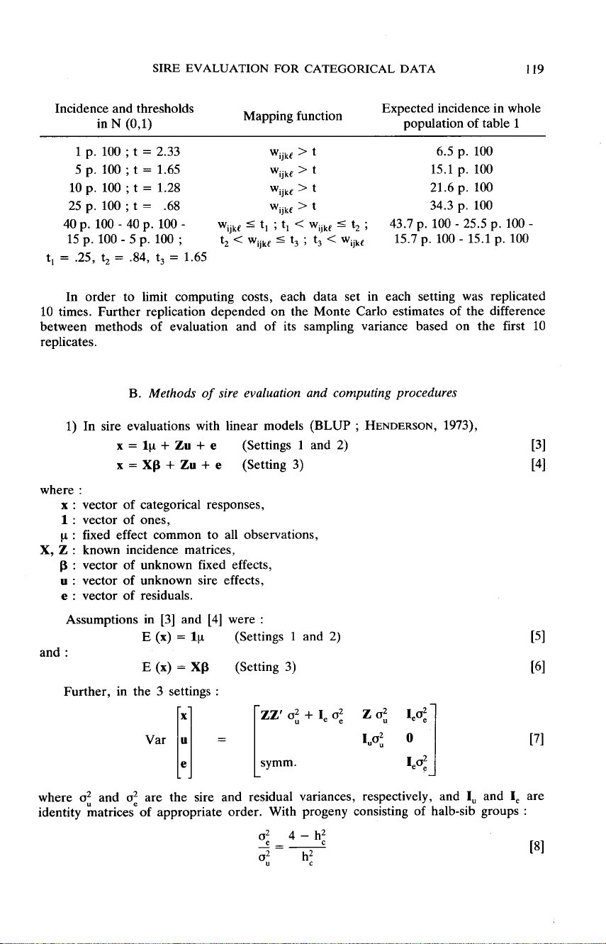
In
order
to
limit
computing
costs,
each
data
set
in
each
setting
was
replicated
10
times.
Further
replication
depended
on
the
Monte
Carlo
estimates
of
the
difference
between
methods
of
evaluation
and
of
its
sampling
variance
based
on
the
first
10
replicates.
B.
Methods
of
sire
evaluation
and
computing
procedures
1)
In
sire
evaluations
with
linear
models
(BLUP ;
H
ENDERSON
,
1973),
where :
x :
vector
of
categorical
responses,
1 :
vector
of
ones,
p :
fixed
effect
common
to
all
observations,
X,
Z :
known
incidence
matrices,
0 :
vector
of
unknown
fixed
effects,
u :
vector
of
unknown
sire
effects,
e :
vector
of
residuals.
and :
Further,
in
the
3
settings :
where
02
and
G2
are
the
sire
and
residual
variances,
respectively,
and 1
.
and
Ie
are
identity
matrices of
appropriate
order.
With
progeny
consisting
of
halb-sib
groups :


![Bộ Thí Nghiệm Vi Điều Khiển: Nghiên Cứu và Ứng Dụng [A-Z]](https://cdn.tailieu.vn/images/document/thumbnail/2025/20250429/kexauxi8/135x160/10301767836127.jpg)
![Nghiên Cứu TikTok: Tác Động và Hành Vi Giới Trẻ [Mới Nhất]](https://cdn.tailieu.vn/images/document/thumbnail/2025/20250429/kexauxi8/135x160/24371767836128.jpg)


