Section on Special Construction Engineering - Vol. 07, No. 02 (Dec. 2024)
150
DAMAGE DETECTION IN STEEL BEAMS THROUGH NATURAL
FREQUENCY USING A RANDOM FOREST MODEL
Van Tuan Vu1,*, Anh Dung Dang1, Hai Dang Lam1,
Duc Thinh Nguyen1, Trung Duc Tran1
1Institute of Techniques for Special Engineering, Le Quy Don Technical University
Abstract
Recently, machine learning (ML) algorithms have proven to be highly effective tools for
predicting structural damage. However, the data used in structural health monitoring often
consists primarily of normal operational conditions or slight deviations from the original
state, with a scarcity of data representing potentially dangerous conditions. This limitation
makes it challenging to create realistic datasets for training ML models to detect structural
damage. If such data were available, it would likely involve parameters like the stress
intensity factor range and stress ratio, which are difficult to measure in real-world structures.
In this study, a random forest (RF) model was developed to predict the locations, widths, and
depths of saw-cuts in steel beams based on variations in natural frequencies. These natural
frequencies under various damage scenarios were determined using the Finite Element
Method (FEM). To ensure accuracy, the natural frequencies in the undamaged state were
compared between the FEM and Frequency Domain Decomposition (FDD). After training,
the RF model showed an R-squared value of 0.996 for location, 0.876 for width, and 0.880
for depth. The mean squared error (MSE) was found to be 0.0003 for location, 0.0313 for
width, and 0.0420 for depth. The results indicate that combining the FEM and FDD with the
RF model holds significant potential for applications in structural health monitoring.
Keywords: Saw-cut prediction; random forest; natural frequency; Frequency Domain
Decomposition; FEM dynamic analysis.
1. Introduction
Beams have long been fundamental in engineering applications and are frequently
used to model civil engineering challenges. Numerous models and techniques have been
developed to detect damage in beams. For instance, Yang et al. [1] applied Galerkin’s
method and the energy approach to identify cracks in vibrating beams. In another study,
Swamidas et al. [2] employed both Timoshenko and Euler formulations to detect cracks
in beams. Research by G. R. Gillich et al. [3], Zhou et al. [4] and G. R. Gillich et al. [5]
focused on detecting damage cracks through vibration measurements. Additionally,
Zhou et al. [6] explored the forced vibration behavior of cracked beams. The findings from
these studies have shown strong performance in structural damage detection.
* Corresponding author, email: vantuanvu@lqdtu.edu.vn
DOI: 10.10.56651/lqdtu.jst.v7.n02.878.sce

Journal of Science and Technique - ISSN 1859-0209
151
In recent years, machine learning algorithms have emerged as powerful tools for
predicting structural damage. Samir et al. [7] addressed damage identification by
employing a Genetic Algorithm (GA) approach that capitalizes on changes in natural
frequencies. Ghadimi et al. [8] developed a crack detection technique using a modified
extreme learning machine, which takes mode shapes and the first three frequencies as
inputs to identify cracks as outputs. This method was tested on several examples and
demonstrated effectiveness, even in the presence of noise. N. Gillich et al. [9] developed
databases with scenarios depicting damage to a cantilever beam, considered crack
location and severity in two steps using ANN and RF, and achieved highly accurate
results in simulations and experiments.
T. C. Le et al. [10] proposed a hybrid approach using Particle Swarm Optimization
(PSO) and Support Vector Machines (SVM) for precise damage identification. This
method eliminated unnecessary parameters by leveraging PSO’s search capabilities and
utilized the robust SVM model to predict damage locations and severity, showing superior
performance compared to other machine learning models, especially in cases of minor
damage. Rathod et al. [11] developed models for damage classification based on the
behavior of mode conversion versus frequency curves for four wave modes. Their
findings highlighted that SVM and RF classifiers excelled in accuracy on the dataset,
achieving the lowest error rates. More recently, de Sousa et al. [12] introduced a machine
learning approach for monitoring structural integrity in beam-like structures, assessing
the effectiveness of six algorithms, including SVM, k-nearest neighbors (kNN), Decision
Tree (DT), Naive Bayes (NB), and RF. Their methodology achieved up to 100% accuracy
with simulated data and 95% accuracy with experimental data, effectively classifying the
health condition of the structures.
It is evident that using machine learning algorithms to predict damage is entirely
feasible and yields very high accuracy. However, in structural health monitoring, the input
data typically represents normal operational conditions or states with minor deviations
from the baseline, lacking information from potentially dangerous conditions. This
absence makes it challenging to develop a realistic dataset for machine learning models
aimed at detecting structural damage. If such data were accessible, it would likely include
parameters such as the stress intensity factor range and stress ratio, which are challenging
to measure accurately in real-world structures.
As a possible approach, numerical models can be employed to generate training
datasets. Machine learning models can then utilize monitoring data from actual structures
to predict beam damage. In this study, a RF model was developed to estimate the
locations, widths, and depths of saw-cuts in steel beams by analyzing variations in natural

Section on Special Construction Engineering - Vol. 07, No. 02 (Dec. 2024)
152
frequencies. These frequencies, corresponding to different damage scenarios, were
determined using a Finite Element Method (FEM) model. To evaluate the viability of this
approach, the natural frequencies without saw-cuts, derived from the Frequency Domain
Decomposition (FDD) method, were compared with those obtained from the FEM.
Conclusions on the integration of FEM, FDD, and the RF model will be drawn
upon completion.
2. Determination of natural frequencies using Frequency Domain
Decomposition and Finite Element Method
2.1. Identification of natural frequencies in a steel beam through Frequency
Domain Decomposition
Brincker et al. [13] introduced the concept of FDD. This approach utilizes singular
value decomposition (SVD) to break down the spectral density matrix at each frequency
into singular values and corresponding singular vectors. FDD is essentially an
enhancement of the traditional frequency domain method, often referred to as the peak
picking technique, where natural frequencies are determined by identifying peaks within
the spectral density matrix.
The connection between the unknown input x(t) and the observed response output
y(t) can be represented by the following equation:
*
[ ( )] [ ( )] [ ( )][ ( )]T
yy xx
G H G H
(1)
where
[ ( )]
xx
G
is the Power Spectral Density (PSD) matrix of the input,
[ ( )]
yy
G
is the
PSD matrix of the responses,
*
[ ( )]H
is the complex conjugate matrix of Frequency
Response Function (FRF),
[ ( )]T
H
is the transpose matrix of FRF.
The FRF can be written in prutial fraction:
*
*
1
[ ] [ ]
[ ( )]
N
kk
kk
RR
Hjj
(2)
k k dk
j
(3)
where N is the number of modes,
k
is the pole of the
th
k
mode shape,
k
is minus the
real part of the pole,
dk
is the damped natural frequencies of the
th
k
mode shape.
[]
k
R
is the residue, defined as follows:
[] T
k k k
R
(4)
where
k
is mode shape vector,
k
is the modal participation vector.

Journal of Science and Technique - ISSN 1859-0209
153
Suppose the input is white noise, its power spectral density is constant or
[ ( )]
xx
G
= C. Formula (1) is rewritten as follows:
**
**
11
[ ] [ ] [ ] [ ]
[ ( )]
T
NN
k k k k
yy
k k k k
R R R R
GC
j j j j
(5)
By multiplying the two partial fraction components and applying the Heaviside
partial fraction theorem, the output PSD can be simplified into a pole/residue form after
some mathematical manipulations, as shown below:
**
**
1
[ ] [ ] [ ] [ ]
[ ( )]
N
k k k k
yy
k k k k
A A B B
Gj j j j
(6)
where
[]
k
A
is the
th
k
residue matrix of the output PSD.
At a specific frequency ω, usually only a few modes, often just one or two, will
have a significant impact. Therefore, for a lightly damped structure, the response spectral
density can generally be expressed as follows:
***
*
()
[ ( )]
TT
k k k k k k
yy
k Sub kk
dd
Gjj
(7)
where
k
∈
Sub(ω) is the set of modes be denoted at a specific frequency.
The FDD method relies on performing a singular value decomposition of the
Hermitian response spectral density matrix.
[ ( )] [ ][ ][ ]H
yy
G U S U
(8)
where
[]S
denotes a diagonal matrix containing the scalar singular values,
[]U
represents
a unitary matrix with the singular vectors, and
[]
H
U
is a Hermitian matrix.
Using vibration measurement data (acceleration) from the structure, we compute
the spectral density matrix
[ ( )]
yy
G
and apply singular value decomposition based on
formula (8) to identify the natural frequencies of the structure.
The test involved capturing dynamic responses (acceleration) of steel beam
structures at various nodes over time. The resulting vibration data was used to determine
the natural frequencies of the structure. The physical parameters of the structure are
detailed in Table 1. The testing equipment included the NIcDAQ-9137 and two
accelerometers (PCB 352C68 and PCB 353B33). The accelerometers, used to measure
beam vibrations (Fig. 1), were connected to the NIcDAQ-9137, which was also connected
Section on Special Construction Engineering - Vol. 07, No. 02 (Dec. 2024)
154
to a display (Fig. 1). Data from the accelerometers were collected and displayed using the
NI Signal Express software. For the measurements, parameters were set up, and vibrations
were induced in the structure with a sufficiently large stimulus to ensure it remained in
the elastic range. The data collected included acceleration values recorded over time at
the locations where the accelerometers were installed.
Following the vibration measurements of the structure, acceleration data at various
nodes on the steel girder structure were collected over time. Examples of measurement
data are illustrated in Fig. 2. Using the experimental acceleration data, the power spectral
density was estimated employing Welch’s method, and singular values were resolved
using the SVD algorithm, as described in formula (8). The natural frequencies of the
structure were identified based on the peaks in the power spectral density function. The
identified natural frequencies are presented in Fig. 3.
Fig. 1. Diagram of the test structure layout.
Table 1. Specifications of the steel beam structure
No.
Parameter
Value
Unit
1
Length
710
mm
2
Height
8
mm
3
Width
60
mm
4
Density weight
7850
kg/m3
5
Modulus of elasticity
2.03·105
MPa