Annals of Mathematics
The symplectic sum
formula for Gromov-
Witten invariants
By Eleny-Nicoleta Ionel and Thomas H. Parker

Annals of Mathematics,159 (2004), 935–1025
The symplectic sum formula
for Gromov-Witten invariants
By Eleny-Nicoleta Ionel and Thomas H. Parker*
Abstract
In the symplectic category there is a ‘connect sum’ operation that glues
symplectic manifolds by identifying neighborhoods of embedded codimension
two submanifolds. This paper establishes a formula for the Gromov-Witten in-
variants of a symplectic sum Z=X#Yin terms of the relative GW invariants
of Xand Y. Several applications to enumerative geometry are given.
Gromov-Witten invariants are counts of holomorphic maps into symplectic
manifolds. To define them on a symplectic manifold (X, ω) one introduces
an almost complex structure Jcompatible with the symplectic form ωand
forms the moduli space of J-holomorphic maps from complex curves into X
and the compactified moduli space, called the space of stable maps. One then
imposes constraints on the stable maps, requiring the domain to have a certain
form and the image to pass through fixed homology cycles in X. When the
correct number of constraints is imposed there are only finitely many maps
satisfying the constraints; the (oriented) count of these is the corresponding
GW invariant. For complex algebraic manifolds these symplectic invariants can
also be defined by algebraic geometry, and in important cases the invariants
are the same as the curve counts that are the subject of classical enumerative
algebraic geometry.
In the past decade the foundations for this theory were laid and the in-
variants were used to solve several long-outstanding problems. The focus now
is on finding effective ways of computing the invariants. One useful technique
is the method of ‘splitting the domain’, in which one localizes the invariant to
the set of maps whose domain curves have two irreducible components with
the constraints distributed between them. This produces recursion relations
relating the desired GW invariant to invariants with lower degree or genus.
This paper establishes a general formula describing the behavior of GW in-
variants under the analogous operation of ‘splitting the target’. Because we
*The research of both authors was partially supported by the NSF. The first author was
also supported by a Sloan Research Fellowship.

936 ELENY-NICOLETA IONEL AND THOMAS H. PARKER
work in the context of symplectic manifolds the natural splitting of the target
is the one associated with the symplectic cut operation and its inverse, the
symplectic sum.
The symplectic sum is defined by gluing along codimension two submani-
folds. Specifically, let Xbe a symplectic 2n-manifold with a symplectic (2n−2)-
submanifold V. Given a similar pair (Y,V ) with a symplectic identification
between the two copies of Vand a complex anti-linear isomorphism between
the normal bundles NXVand NYVof Vin Xand in Y, we can form the sym-
plectic sum Z=X#VY. Our main theorem is a ‘Symplectic Sum Formula’
which expresses the GW invariants of the sum Zin terms of the relative GW
invariants of (X, V ) and (Y,V ) introduced in [IP4].
The symplectic sum is perhaps more naturally seen not as a single manifold
but as a family depending on a ‘squeezing parameter’. In Section 2 we construct
a family Z→Dover the disk whose fibers Zλare smooth and symplectic for
λ= 0 and whose central fiber Z0is the singular manifold X∪VY.Ina
neighborhood of V, the total space Zis NXV⊕NYVand the fiber Zλis
defined by the equation xy =λwhere xand yare coordinates in the normal
bundles NXVand NYV∼
=(NXV)∗. The fibration Z→Dextends away from
Vas the disjoint union of X×Dand Y×D, and the entire fibration Zcan be
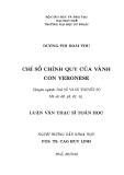
given an almost K¨ahler structure. The smooth fibers Zλ, depicted in Figure 1,
are symplectically isotopic to one another; each is a model of the symplectic
sum.
The overall strategy for proving the symplectic sum formula is to relate
the holomorphic maps into Z0, which are simply maps into Xand Ywhich
match along V, with the holomorphic maps into Zλfor λclose to zero. This
strategy involves two parts: limits and gluing. For the limiting process we
consider sequences of stable maps into the family Zλof symplectic sums as the
‘neck size’ λ→0. In particular, these are stable maps into a compact region
of the almost K¨ahler manifold Z, so that the compactness theorem for stable
maps applies, giving limit maps into the singular manifold Z0obtained by
identifying Xand Yalong V. Along the way several things become apparent.
First, the limit maps are holomorphic only if the almost complex struc-
tures on Xand Ymatch along V. To ensure this we impose the “V-compat-
ibility” condition (1.10) on the almost complex structure. But there is a price
to pay for that specialization. In the symplectic theory of Gromov-Witten
invariants we are free to perturb (J, ν) without changing the invariant; this
freedom can be used to ensure that intersections are transverse. After impos-
ing the V-compatibility condition, we can no longer perturb (J, ν) along Vat
will, and hence we cannot assume that the limit curves are transverse to V.
In fact, the images of the components of the limit maps meet Vat points
with well-defined multiplicities and, worse, some components may be mapped
entirely into V.
THE SYMPLECTIC SUM FORMULA 937
To count stable maps into Z0we look first on the Xside and ignore the
maps which have marked points, double points, or whole components mapped
into V. The remaining “V-regular” maps form a moduli space which is the
union of components MV
s(X) labeled by the multiplicities s=(s1,...,s
ℓ)of
the intersection points with V. We showed in [IP4] how these spaces MV
s(X)
can be compactified and used to define relative Gromov-Witten invariants
GWV
X. The definitions are briefly reviewed in Section 1.
XY
Figure 1. Limiting curves in Zλ=X#λYas λ→0.
Second, as Figure 1 illustrates, connected curves in Zλcan limit to curves
whose restrictions to Xand Yare not connected. For that reason the GW
invariant, which counts stable curves from a connected domain, is not the ap-
propriate invariant for expressing a sum formula. Instead one should work with
the ‘Gromov-Taubes’ invariant GT, which counts stable maps from domains
that need not be connected. Thus we seek a formula of the general form
GTV
X∗GTV
Y=GT
Z
(0.1)
where ∗is some operation that adds up the ways curves on the Xand Y
sides match and are identified with curves in Zλ. That necessarily involves
keeping track of the multiplicities sand the homology classes. It also involves
accounting for the limit maps with nontrivial components in V; such curves
are not counted by the relative invariant and hence do not contribute to the
left side of (0.1). We postpone this issue by first analyzing limits of curves
which are δ-flat in the sense of Definition 3.1.
A more precise analysis reveals a third complication: the squeezing process
is not injective. In Section 5 we again consider a sequence of stable maps fn
into Zλas λ→0, this time focusing on their behavior near V, where the fndo
not uniformly converge. We form renormalized maps ˆ
fnand prove that both
the domains and the images of the renormalized maps converge. The images
converge nicely according to the leading order term of their Taylor expansions,
but the domains converge only after we fix certain roots of unity.
These roots of unity are apparent as soon as one writes down formulas.
Each stable map f:C→Z0decomposes into a pair of maps f1:C1→X
and f2:C2→Ywhich agree at the nodes of C=C1∪C2. For a specific
example, suppose that fis such a map that intersects Vat a single point p
938 ELENY-NICOLETA IONEL AND THOMAS H. PARKER
with multiplicity three. Then we can choose local coordinates zon C1and w
on C2centered at the node, and coordinates xon Xand yon Yso that f1
and f2have expansions x(z)=az3+··· and y(w)=bw3+···. To find maps
into Zλnear f, we smooth the domain Cto the curve Cµgiven locally near
the node by zw =µand require that the image of the smoothed map lie in Zλ,
which is locally the locus of xy =λ. In fact, the leading terms in the formulas
for f1and f2define a map F:Cµ→Zλwhenever
λ=xy =az3·bw3=ab (zw)3=ab µ3
and conversely every family of smooth maps which limit to fsatisfies this
equation in the limit (cf. Lemma 5.3). Thus λdetermines the domain Cµup
to a cube root of unity. Consequently, this particular fis, at least a priori,
close to three smooth maps into Zλ— a ‘cluster’ of order three.
Other maps finto Z0have larger associated clusters (the order of the
cluster is the product of the multiplicities with which fintersects V). The
maps within a cluster have the same leading order formula but have different
smoothings of the domain. As λ→0 the cluster coalesces, limiting to the
single map f.
This clustering phenomenon greatly complicates the analysis. To distin-
guish the curves within each cluster and make the analysis uniform in λas
λ→0, it is necessary to use ‘rescaled’ norms and distances which magnify
distances as the clusters form. With the right choice of norms, the distances
between the maps within a cluster are bounded away from zero as λ→0 and
become the fiber of a covering of the space of limit maps. Sections 4–6 in-
troduce the required norms, first on the space of curves, then on the space of
maps.
For maps we use a Sobolev norm weighted in the directions perpendicular
to V; the weights are chosen so the norm dominates the C0distance between
the renormalized maps ˆ
f. On the space of curves we require a stronger metric
than the usual complete metrics on Mg,n. In Section 4 we define a complete
metric on Mg,n \N where Nis the set of all nodal curves. In this metric
the distance between two sequences that approach Nfrom different directions
(corresponding to the roots of unity mentioned above) is bounded away from
zero; thus this metric separates the domain curves of maps within a cluster.
This construction also leads to a compactification of Mg,n \N in which the
stratum Nℓof ℓ-nodal curves is replaced by a bundle over Nℓwhose fiber is
the real torus Tℓ.
The limit process is reversed by constructing a space of approximately
holomorphic maps and showing it is diffeomorphic to the space of stable maps
into Zλ. The space of approximate maps is described in Section 6, first in-
trinsically, then as a subset Models(Zλ) of the space of maps. For each sand
λit is a covering of the space Ms(Z0) of the δ-flat maps into Z0that meet


![Luận văn Thạc sĩ Toán học: Chứng minh định lý bất biến Dickson của Steinberg [chuẩn nhất]](https://cdn.tailieu.vn/images/document/thumbnail/2024/20241209/myhouse02/135x160/3741733678218.jpg)