
80 •Chapter 10
particular, the individual typically has some influence on the outcome.
Thus, the probability q, which was taken as given, may be regarded, to
some extent at least, as influenced by individual decisions that involve
costs and efforts. The potential conflict that this type of moral hazard
raises between social welfare and individual interests is very clear in this
context. Since V∗
1<V∗
2,an increase in q decreases the first-best expected
utility. On the other hand, in a competitive equilibrium, ˆ
V
1>ˆ
V
2,and
hence an increase in qmay be desirable.

CHAPTER 9
Pooling Equilibrium and Adverse Selection
9.1Introduction
For a competitive annuity market with long-term annuities to be efficient,
it must be assumed that individuals can be identified by their risk classes.
We now wish to explore the existence of an equilibrium in which the
individuals’ risk classes are unknown and cannot be revealed by their
actions. This is called a pooling equilibrium.
Annuities are offered in a pooling equilibrium at the same price to
all individuals (assuming that nonlinear prices, which require exclusivity,
as in Rothschild and Stiglitz (1979), are not feasible). Consequently,
the equilibrium price of annuities is equal to the average longevity of the
annuitants, weighted by the equilibrium amounts purchased by different
risk classes. This result has two important implications. One, the amount
of annuities purchased by individuals with high longevity is larger than in
a separating, efficient equilibrium, and the opposite holds for individuals
with low longevities. This is termed adverse selection. Two, adverse
selection causes the prices of annuities to exceed the present values of
expected average actuarial payouts.
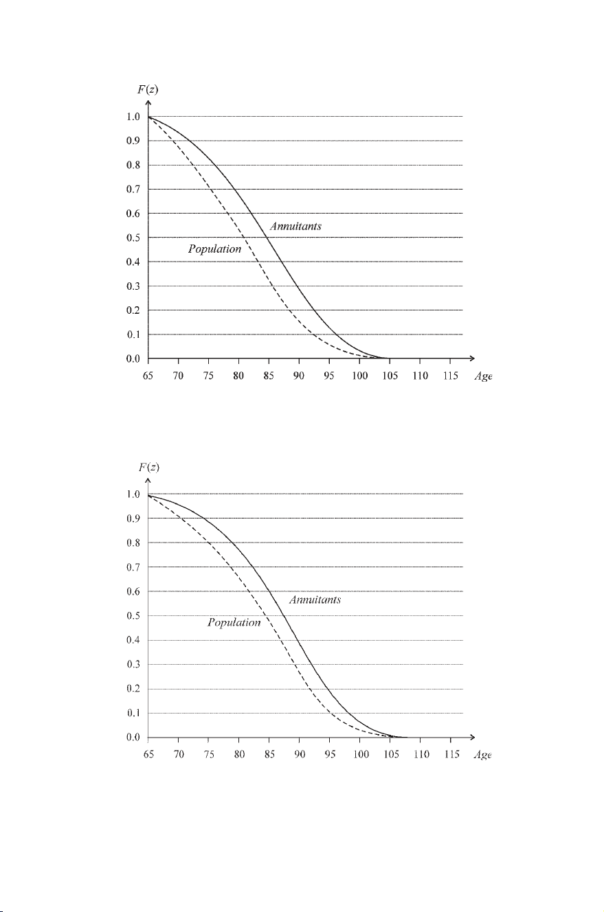
The empirical importance of adverse selection is widely debated
(see, for example, Chiapori and Salanie (2000), though its presence is
visible. For example, from the data in Brown et al. (2001), one can
derive survival rates for males and females born in 1935, distinguish-
ing between the overall population average rates and the rates appli-
cable to annuitants, that is, those who purchase private annuities. As
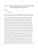
figures 9.1(a) and (b) clearly display, at all ages annuitants, whether
males or females, have higher survival rates than the population average
rates (table 9A.1 in the appendix provides the underlying data). Adverse
selection seems somewhat smaller among females, perhaps because of the
smaller variance in female survival rates across different occupations and
educational groups.
Adverse selection may be reflected not only in the amounts of annuities
purchased by different risk classes but also in the selection of different
insurance instruments, such as different types of annuities. We explore
this important issue in chapter 11.
(a)
Z
Figure 9.1(a). Male survival functions (1935 cohort). (Source: Brown et al. 2001,
table 1.1).
(b)
Z
Figure 9.1(b). Female survival functions (1935 cohort). (Source: Brown et al.
2001, table 1.1).

Pooling Equilibrium •69
9.2General Model
We continue to denote the flow of returns on long-term annuities
purchased prior to age Mby r(z),M≤z≤T.
The dynamic budget constraint of a risk-class-iindividual, i=1,2,
is now
˙
ai(z)=rp(z)ai(z)+w(z)−ci(z)+r(z)a(M),M≤z≤T,(9.1)
where ˙
ai(z) are annuities purchased or sold (with ai(M)=0) and rp(z)
is the rate of return in the (pooled) annuity market for age-zindividuals,
M≤z≤T.
For any consumption path, the demand for annuities is, by (9.1),
ai(z)=exp z
M
rp(x)dxz
M
exp −x
M
rp(h)dh
×(w(x)−ci(x)+r(x)a(M)) dx,i=1,2.(9.2)
Maximization of expected utility,
T
M
Fi(z)u(ci(z)) dz,i=1,2,(9.3)
subject to (9.1) yields optimum consumption, denoted ˆ
ci(z),
ˆ
ci(z)=ˆ
ci(M) exp z
M
1
σ(rp(x)−ri(x)) dx,M≤z≤T,i=1,2
(9.4)
(where σis evaluated at ˆ
ci(x)). It is seen that ˆ
ci(z) increases or decreases
with age depending on the sign of rp(z)−ri(z).Optimum consumption
at age M,ci(M),is found from (9.2), setting ai(T)=0,
T
M
exp −x
M
rp(h)dh(w(x)−ˆ
ci(x)+r(x)a(M)) dx =0,i=1,2.
(9.5)
Substituting for ˆ
ci(x),from (9.4),
ˆ
ci(M)=T
Mexp −x
Mrp(h)dh(w(x)+r(x)a(M)) dx
T
Mexp x
M
1
σ((1 −σ)rp(h)−ri(h)) dhdx ,i=1,2.(9.6)

70 •Chapter 9
Since r1(z)<r2(z) for all z,M≤z≤T,it follows from (9.6) that
ˆ
c1(M)<ˆ
c2(M).Inserting optimum consumption ˆ
ci(x) into (9.2), we
obtain the optimum demand for annuities, ˆ
ai(z).
Since ˆ
ai(M)=0,it is seen from (9.1) that ˙
ˆ
a1(M)>˙
ˆ
a2(M). In fact, it
can be shown (see appendix) that ˆ
a1(z)>ˆ
a2(z) for all M<z<T.
This is to be expected: At all ages, the stochastically dominant risk
class, having higher longevity, holds more annuities compared to the risk
class with lower longevity.
We wish to examine whether there exists an equilibrium pooling
rate of return, rp(z),that satisfies the aggregate resource constraint
(zero expected profits). Multiplying (9.1) by Fi(z) and integrating by
parts, we obtain
T
M
Fi(z)(rp(z)−ri(z)) ˆ
ai(z)dz
=T
M
Fi(z)(w(z)−ˆ
ci(z))dz +aMT
M
r(z)dz,i=1,2.(9.7)
Multiplying (9.7) by pfor i=1 and by (1 −p)fori=2,and adding,
T
M
[(pF1(z)ˆ
a1(z)+(1 −p)F2(z)ˆ
a2(z))rp(z)
−(pF1(z)ˆ
a1(z)r1(z)+(1 −p)F2(z)ˆ
a2(z)r2(z))]dz
=pT
M
F1(z)(w(z)−ˆ
c1(z)) dz +(1 −p)M
T
F2(z)(w(z)−ˆ
c2(z)) dz
+a(M)T
M
(pF1(z)+(1 −p)F2(z))r(z)dz.(9.8)
Recall that
r(z)=pF1(z)r1(z)+(1 −p)F2(z)r2(z)
pF1(z)+(1 −p)F2(z)
is the rate of return on annuities purchased prior to age M. Hence
the last term on the right hand side of (9.8) is equal to F(M)a(M)=
M
0F(z)(w(z)−c)dz.Thus, the no-arbitrage condition in the pooled


![Tín dụng trung-dài hạn: Những vấn đề cơ bản [chuẩn nhất]](https://cdn.tailieu.vn/images/document/thumbnail/2013/20131120/butmauden/135x160/6441384999291.jpg)


![Đề thi giữa học kì Tài chính tiền tệ: Tổng hợp [Năm]](https://cdn.tailieu.vn/images/document/thumbnail/2026/20260513/hoacattuong2026/135x160/81291778835177.jpg)


%20--%3e%3cdefs%3e%3cstyle%3e%20.st0%20{%20fill:%20%23fff;%20}%20.st1%20{%20fill:%20%237800fa;%20}%20%3c/style%3e%3c/defs%3e%3cpath%20class='st1'%20d='M117.78,12.18H43.11c2.9,3.47,4.65,7.94,4.65,12.82,0,5.6-2.3,10.66-6.01,14.29h76.02l7.22-13.56-7.22-13.56Z'/%3e%3cg%3e%3cpath%20class='st0'%20d='M53.58,26.17h-.59v-1.46h.59v-4.96h2.83c1.78,0,2.67.94,2.67,2.82v5.76c0,1.87-.89,2.81-2.67,2.81h-2.83v-4.96ZM55.36,21.37v3.34h1.1v1.46h-1.1v3.34h1.01c.61,0,.91-.37.91-1.1v-5.93c0-.74-.3-1.1-.91-1.1h-1.01Z'/%3e%3cpath%20class='st0'%20d='M65.99,31.14h-1.8l-.31-2.07h-2.19l-.31,2.07h-1.64l1.82-11.39h2.62l1.82,11.39ZM65.28,18.04c-.25.46-.51.77-.75.94-.21.15-.47.22-.79.22-.26,0-.57-.07-.92-.22l-.38-.15c-.14-.05-.26-.07-.37-.07-.3,0-.53.18-.71.54l-.91-.68c.25-.46.51-.77.75-.94.21-.14.48-.21.79-.21.26,0,.57.07.92.21l.38.15c.14.05.26.07.37.07.3,0,.53-.18.71-.54l.91.68ZM61.91,27.52h1.73l-.87-5.76-.87,5.76Z'/%3e%3cpath%20class='st0'%20d='M74.53,26.89v1.52c0,1.91-.89,2.86-2.67,2.86s-2.67-.95-2.67-2.86v-5.93c0-1.91.89-2.86,2.67-2.86s2.67.95,2.67,2.86v1.11h-1.69v-1.22c0-.75-.31-1.12-.93-1.12s-.93.37-.93,1.12v6.15c0,.74.31,1.11.93,1.11s.93-.37.93-1.11v-1.63h1.69Z'/%3e%3cpath%20class='st0'%20d='M81.4,31.14h-1.8l-.31-2.07h-2.19l-.31,2.07h-1.64l1.82-11.39h2.62l1.82,11.39ZM75.9,19.2l1.52-1.91h1.71l1.51,1.91h-1.61l-.76-.95-.75.95h-1.61ZM77.32,27.52h1.73l-.87-5.76-.87,5.76ZM83.1,15.99l-1.76,1.91h-1.26l1.17-1.91h1.86Z'/%3e%3cpath%20class='st0'%20d='M84.86,19.75c1.78,0,2.67.94,2.67,2.82v1.48c0,1.87-.89,2.81-2.67,2.81h-.85v4.28h-1.79v-11.39h2.64ZM84.01,21.37v3.86h.85c.58,0,.87-.36.87-1.08v-1.71c0-.71-.29-1.07-.87-1.07h-.85Z'/%3e%3cpath%20class='st0'%20d='M93.51,19.75c1.78,0,2.67.94,2.67,2.82v1.48c0,1.87-.89,2.81-2.67,2.81h-.85v4.28h-1.79v-11.39h2.64ZM92.66,21.37v3.86h.85c.58,0,.87-.36.87-1.08v-1.71c0-.71-.29-1.07-.87-1.07h-.85Z'/%3e%3cpath%20class='st0'%20d='M98.8,31.14h-1.79v-11.39h1.79v4.88h2.03v-4.88h1.83v11.39h-1.83v-4.88h-2.03v4.88Z'/%3e%3cpath%20class='st0'%20d='M105.36,24.55h2.46v1.62h-2.46v3.34h3.09v1.63h-4.88v-11.39h4.88v1.63h-3.09v3.18ZM108.17,17.29l-1.76,1.91h-1.26l1.17-1.91h1.86Z'/%3e%3cpath%20class='st0'%20d='M112.2,19.75c1.78,0,2.67.94,2.67,2.82v1.48c0,1.87-.89,2.81-2.67,2.81h-.85v4.28h-1.79v-11.39h2.64ZM111.35,21.37v3.86h.85c.58,0,.87-.36.87-1.08v-1.71c0-.71-.29-1.07-.87-1.07h-.85Z'/%3e%3c/g%3e%3ccircle%20class='st1'%20cx='25'%20cy='25'%20r='20'/%3e%3cpath%20class='st0'%20d='M32.78,19.27c2.92,0,4.43,2.55,5.28,5.33l.71,2.17c.14.38-.33.75-.71.75h-5.61c.19-.33.24-.71.09-1.08l-.75-2.45c-.43-1.32-.99-2.64-1.79-3.77.75-.57,1.65-.94,2.78-.94h0ZM25,18.38c3.25,0,4.9,2.78,5.89,5.89l.76,2.45c.14.42-.33.8-.8.8h-11.69c-.42,0-.94-.38-.8-.8l.75-2.45c.99-3.11,2.64-5.89,5.89-5.89h0ZM25,11.35c1.74,0,3.11,1.37,3.11,3.11s-1.37,3.11-3.11,3.11-3.11-1.41-3.11-3.11,1.41-3.11,3.11-3.11h0ZM17.27,19.27c1.08,0,1.98.38,2.73.94-.8,1.13-1.37,2.45-1.74,3.77l-.8,2.45c-.14.38-.05.75.09,1.08h-5.56c-.42,0-.9-.38-.75-.75l.71-2.17c.9-2.78,2.41-5.33,5.33-5.33h0ZM17.27,12.91c1.51,0,2.78,1.27,2.78,2.83s-1.27,2.83-2.78,2.83-2.83-1.27-2.83-2.83,1.27-2.83,2.83-2.83h0ZM32.78,12.91c1.56,0,2.78,1.27,2.78,2.83s-1.23,2.83-2.78,2.83-2.83-1.27-2.83-2.83,1.27-2.83,2.83-2.83h0ZM27.07,28.56v.09c0,.57-.24,1.08-.61,1.46h0v.05c-.38.33-.9.57-1.46.57s-1.08-.24-1.46-.61h0c-.38-.38-.61-.9-.61-1.46v-.09h1.41v.09c0,.19.05.38.19.47v.05c.09.09.28.19.47.19s.38-.09.47-.19v-.05c.14-.09.24-.28.24-.47t-.05-.09h1.41ZM30.99,28.56v.09c0,1.65-.66,3.16-1.74,4.24-1.08,1.08-2.59,1.79-4.24,1.79s-3.16-.71-4.24-1.79l-.05-.05c-1.04-1.08-1.7-2.55-1.7-4.2v-.09h1.41v.09c0,1.27.47,2.4,1.27,3.25h.05c.85.85,1.98,1.37,3.25,1.37s2.4-.52,3.25-1.37c.85-.8,1.37-1.98,1.37-3.25v-.09h1.37ZM34.99,28.56v.09c0,2.78-1.13,5.28-2.92,7.07-1.79,1.79-4.29,2.92-7.07,2.92s-5.23-1.13-7.07-2.92c-1.79-1.79-2.92-4.29-2.92-7.07v-.09h1.41v.09c0,2.4.94,4.53,2.5,6.08,1.56,1.56,3.72,2.5,6.08,2.5s4.52-.94,6.08-2.5c1.56-1.56,2.5-3.68,2.5-6.08v-.09h1.41Z'/%3e%3c/svg%3e)