
* Corresponding author.
E-mail addresses: msafarabadi@ut.ac.ir (M. Safarabadi)
© 2018 by the authors; licensee Growing Science, Canada.
doi: 10.5267/j.esm.2017.11.004
Engineering Solid Mechanics (2018) 11-20
Contents lists available at GrowingScience
Engineering Solid Mechanics
homepage: www.GrowingScience.com/esm
Finite element prediction of curing micro-residual stress distribution in polymeric
composites considering hybrid interphase region
V. Teimouri and M. Safarabadi*
School of Mechanical Engineering, College of Engineering, University of Tehran, Tehran 11365-4563, Iran
A R T I C L EI N F O A B S T R A C T
Article history:
Received 26 August, 2017
Accepted 20 November 2017
Available online
20 November 2017
The interphase is a region between fibers and a matrix, which has different properties from the
matrix and the fibers, but is dependent on them. Considering the interphase region has a
significant effect on the accuracy of obtained residual stresses. So far, in order to obtain the
micromechanical residual stresses, the interphase properties are considered as an average. In
this paper, the properties of the interphase are assumed variable by using a suitable UMAT
code in the ABAQUS software. The equations of previous studies that have acquired
interphase properties to be variable are used to write the UMAT code. A representative volume
element (RVE) in polymer composites is modeled in three phases in the ABAQUS software
and the interphase properties are considered as FGM by using the UMAT code. Temperature
variation during curing to environment temperature is the only loading factor in the RVE. The
matrix, fiber and interphase stresses are obtained in the ABAQUS software. The achieved
stresses were compared with the results of previous studies that considered interphase
properties as average. Finite element and energy methods were used in previous papers but in
the present study just the finite element method with variable interphase properties was use. In
addition, residual stress diagrams with the variable interphase properties are plotted to study
the effect of the thermal expansion coefficient. The results of this study are similar to those in
previous ones, and the curves are improved.
© 2018 b
y
the authors; licensee Growin
g
Science, Canada.
Keywords:
Finite element simulation
UMAT code
Interphase
Variable properties
Residual micromechanical stress
1. Introduction
Residual stress is the stress that exists in the body, without the body being under external load or
temperature gradients. In composite materials, after the curing process, their temperature decreases
from the curing temperature to the environment temperature. Because of the incompatibility between
the fibers and matrix thermal expansion coefficients, residual stresses will form (Ghasemi, 2007).
Residual stresses have a major effect on the properties of composites. These stresses cause the forming

12
of cracks in the matrix, the layering of the structure, breaking of the fibers and the fluctuation of the
asymmetric multi-layers and have a significant effect on reducing the final stability of the structure.
There are different numerical methods such as finite element, finite difference, boundary element and
finite volume to solve engineering problems. Considering previous research, the finite element method
is the most widely used method for determining residual stresses in multi-layer composites. Chen et al.
(2001) investigated the non-linear viscoelasticity of the matrix in the formation of residual stresses in
a multi-layer composite [0/90] by using a finite element model at a micro scale. The results of the finite
element analysis showed that the higher the cooling rate, the taller the layers in residual stress will be.
Also the effect of the free edge surface on the formation of residual stresses was investigated in this
analysis. Tay and shen (2002) used a cracked finite element model to investigate the effect of residual
stresses in layering and buckling of the layers. According to their research, the residual stress has a
significant effect on the initiation of the buckling of the layered sub layer, but does not have any effect
on the rate of local strain energy release during post-buckling. Karami and Garnich (2003) considered
the fibers wavy form in their finite element model. Considering this issue, the thermal expansion
coefficient changes as the fiber is assumed to be direct, but the amount of residual stress does not
change.
Zhang et al. (2003) developed a finite element model similar to the Chen model to investigate the
residual stresses during and after high-temperature curing. Based on their results, after the cooking
process, the residual stresses decreases over time, and after about 34 hours, a small amount is reached.
Aghdam and Khojeh (2003) studied the role of residual stresses in the stress-strain curve of a
unidirectional composite under tensile longitudinal loads by considering a square-shaped element, and
compared the results of the finite element solution with experimental results. Hobbiebrunken et al.
(2005) performed a nonlinear finite element analysis, considering a RVE. Based on their results, a high
residual shear stress during curing, causes local yield in the matrix which causes a new distribution of
stress and thus lower residual stresses compared to a linear elastic matrix. The results show local yield
of the matrix leads to lower stress concentration. Using a viscoelastic model in the micro scale, Zhao
et al. (2006) assessed residual stresses in a glass-epoxy composite. Due to the viscoelastic behavior of
the matrix, part of the residual stress is released and hence the residual stress decreases. Considering
similar thermal changes, the amount of this stress is dependent on the fiber volume ratio. These stresses
play a role in lateral and shear damage. Hook et al. (2008), assessed the effect of geometry in effective
material properties and stress distribution considering various finite element models.
Shokrieh and Ghanei (2010) considered a single fiber circular composite to assess residual thermal
stresses in a finite element simulation. The interphase properties were considered to vary cubic,
exponentially and periodically, radially and found that the results coincide with proper boundary
conditions and neglecting the interphase causes obvious errors. Shokrieh and Safarabadi (2011),
utilizing the Energy method and considering average interphase properties found the micromechanical
residual stress in various points of the RVE. They evaluated the effect of the modulus of elasticity,
Poisson’s ration and the thermal expansion coefficient of the interphase on micromechanical residual
stresses. They used ABAQUS CAE considering seven layers for the interphase to compare the results.
Shokrieh and Safarabadi (2012a) have reported that axial and sheer stresses increase not only because
of an increase in the fiber length, but also due to the order of mismatch in thermal and mechanical
properties and high mismatch in coefficient of the thermal expansion and Young’s modulus. By
comparing the theoretical and numerical results together, inability of finite element in elucidation
boundary conditions at the composition ends resolved.
Shokrieh et al. (2012) reported finite-element analysis as a new three-dimensional analytical model,
based on the energy method, is developed to present residual stresses, which is a little higher in
representative volume element (RVE) in polymer composites. Because of not considering the edge
singularity in this method, a maximum shear stress is reached at composite ends in comparison at
vicinity of fiber ends. In this study, first, the interphase properties' equations is found using previous
studies; then a finite element solution is used and micromechanical residual stress curves are plotted
V. Teimouri and M. Safarabadi / Engineering Solid Mechanics 6 (2018)
13
and the results are compared with previous research. Finally, the effect of the mechanical and thermal
properties' bonding efficiencies are evaluated.
2. Micromechanical residual stress distribution prediction using the finite element solution
In this part, first, the interphase equations are found using previous studies. Then the finite element
solution is described. In the finite element solution an appropriate UMAT program is used.
2-1. Interphase property prediction
Initially the interphase properties, which depend on the matrix and fiber properties, need to be
found. Papanicolaou et al. (2002) presented a precise two dimensional model to determine the
micromechanical properties of the interphase under thermal load.
= 111
1
(1)
in which can be the modulus of elasticity, Poison’s ratio and thermal expansion coefficient (Eq 2).
Which is the property mismatch index is found from equation 3. And ρ are the mechanical and
thermal bonding property efficiencies at r= and the normal radial distance with respect to the fiber
radius respectively. Accounts for the geometry and bonding efficiency aspects of the model,
which is found from Eq (4).
=
1
ʋ
ʋ2
3
(2)
=
1
ʋ
ʋ2
3
(3)
=
⁄/
⁄/, (4)
where Eq. (4) and are interphase to fiber radius ratio and anisotropy index respectively.
=
1
ʋ
ʋ2
3
(5)
In Eq. (5), t and l are principal values of material properties along transverse and longitude
directions respectively.
2.2. Residual stress prediction
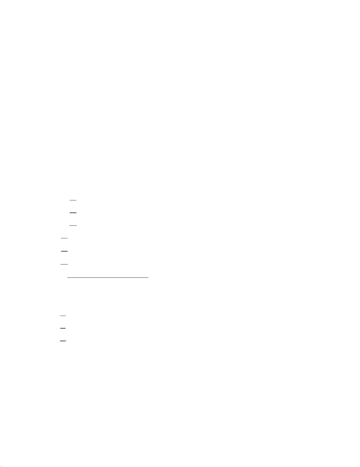
In Fig. 1, the considered RVE for the finite element solution is seen. This RVE is in all three
phases.
14
Fig. 1. RVE considered for predicting micromechanical stresses
The considered composite in this study is glass-epoxy, whose properties have been presented in
Table 1.
Table 1. Glass epoxy composite properties (Shokrieh & Safarabadi, 2012b)
Fiber Matrix Interphase
)(GPa
Young’s modulus 77 3.1 10.2
Poisson’s ratio 0.2 0.34 0.25
)/10(
6
C
Coefficient of thermal expansion 5.4 70 20
)( m
Radius 6 8.5 6.3,6.4,6.7
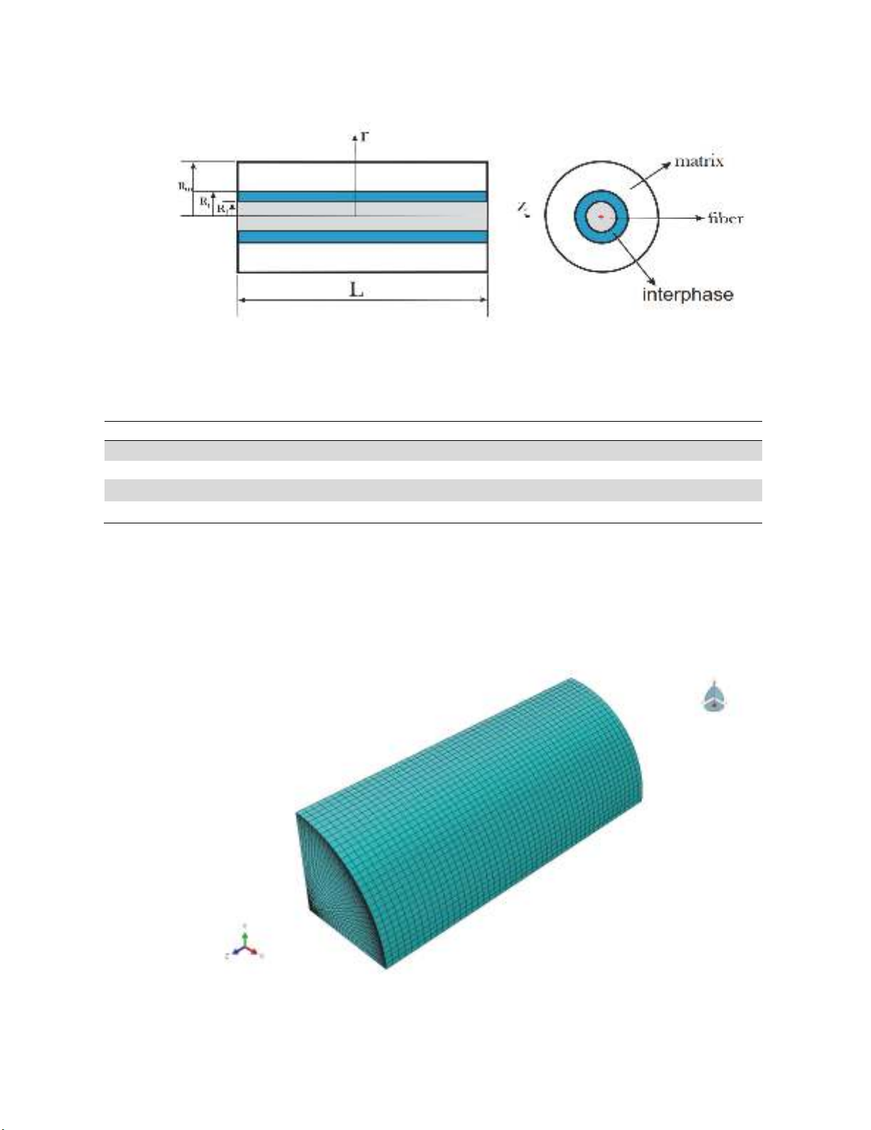
In order to development a numerical model, the finite element model is also assessed. Due to the
geometric symmetry and boundary conditions a quarter of the RVE is modeled and symmetry
constraints are used. The finite element model and its features are shown in Fig. 2 and Table 1
respectively. C3D8R elements were used for meshing the finite element model. In the axial direction
half of the RVE is modelled and one end of the model (which represents the middle of the RVE) is
constrained.
Fig. 2. Finite element model
V. Teimouri and M. Safarabadi / Engineering Solid Mechanics 6 (2018)
15
Table 1. Finite element model parameters
number Type Element
57330
C3D8R Linear hexahedral
1470
C3D6
Number of nodes:62050
Number of elements:58800
Linear wedge
In the finite element model, the interphase properties have been considered to be varying using Eq.
1. To this extent a UMAT program is used to consider varying properties in the radial direction. In this
solution only an 80 degree load is present and there is no constraint.
3. Results and Discussions
The interphase thickness has been found to be 0.3, 0.4 and 0.7 micrometers (Shokrieh & Safarabadi
2011). In this section, first the micromechanical residual stress curves found using the ABAQUS
software for a glass-epoxy composite for different thicknesses are assessed and are compared with
previous studies. The interphase stress curves are also evaluated. Then the thermal expansion bonding
efficiency is discussed.
3.1. Stress distribution in fiber and resin
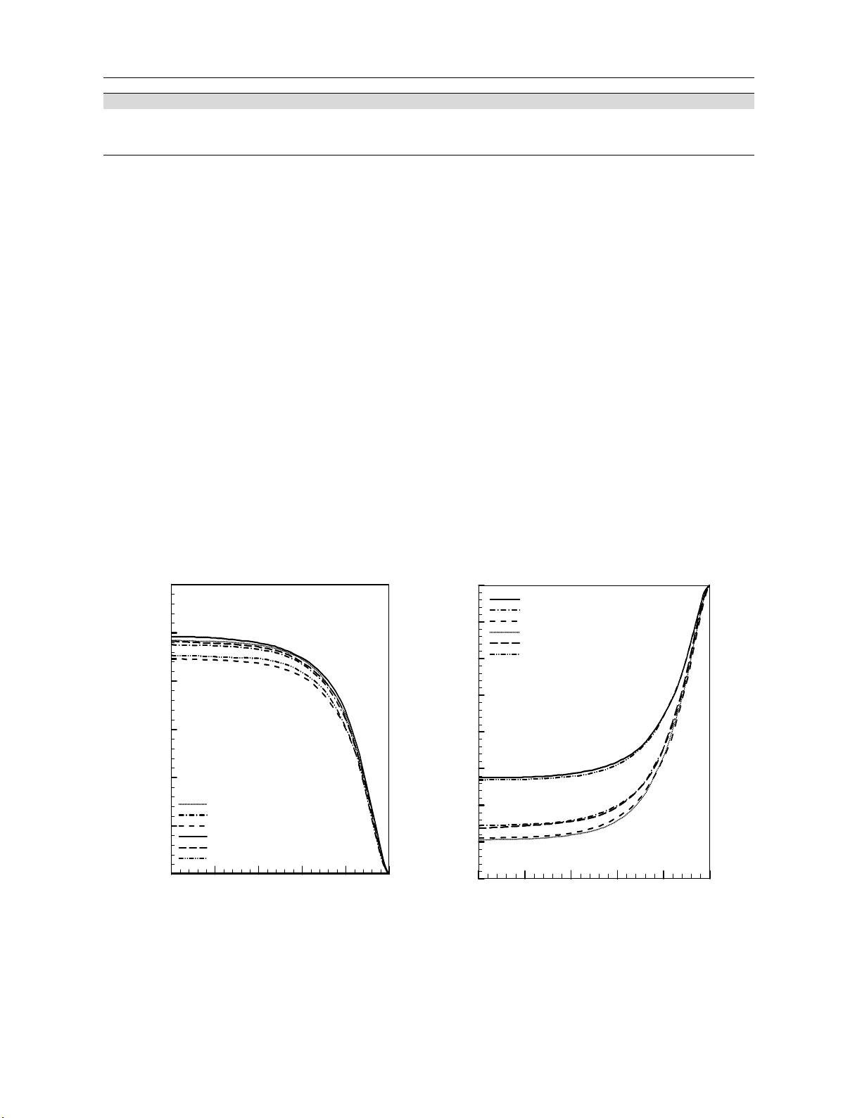
In Fig. 3a, the axial stress distribution in the matrix is shown. As is seen, increasing the interphase
thickness leads to lower stresses. Also, the results found from the finite element solution are higher
than the energy method (Shokrieh & Safarabadi, 2011) considering average properties, but are close.
The maximum stress is in the middle of the RVE, and at the ends the axial stress is zero. Fig. 3b, shows
axial stress distribution in the fiber. Increasing the interphase thickness decreases the amount of stress.
In this section the results are close and the maximum stress is in the middle of the RVE; the stresses at
the ends of the element are zero.
(b) (a)
Fig. 3. axial stress distribution using the finite element solution (considering variable
properties) and the energy method (Shokrieh and Safarabadi, 2011) for different interphase
thicknesses for the matrix (a) and the fiber (b)
Normalized Length(z/l)
Fiber Axial Stress(M Pa)
00.1 0.2 0.3 0.4 0.5
-4
-3.5
-3
-2.5
-2
-1.5
-1
-0.5
0
Energy Method, Interphase Thickness=.7 micrometer
Energy Method, Interphase Thickness=.4 micrometer
Energy Method, Interphase Thickness=.3 micrometer
FEM Analysis, Interphase Thickness=.3 micrometer
FEM Analysis, Interphase Thickness=.4 micrometer
FEM Analysis, Interphase Thickness=.7 micrometer
Normalized Length(z/l)
M a tr ix A xia l Stre ss(M P a )
00.1 0.2 0.3 0.4 0.5
0
0.5
1
1.5
2
2.5
3
Energy Method, Interphase Thickness=.3 micrometer
Energy Method, Interphase Thickness=.4 micrometer
Energy Method, Interphase Thickness=.7 micrometer
FEM Analysis, Interphase Thickness=.3 micrometer
FEM Analysis, Interphase Thickness=.4 micrometer
FEM Analysis, Interphase Thickness=.7 micrometer


![Giáo trình Cấu trúc dữ liệu và giải thuật - Trường CĐ Cơ điện Hà Nội [Mới nhất]](https://cdn.tailieu.vn/images/document/thumbnail/2026/20260323/lionelmessi01/135x160/58171774381670.jpg)


![Giáo trình Tiện nâng cao (Nghề Cắt gọt kim loại, Trình độ Cao đẳng) - Trường Cao đẳng Cơ điện Hà Nội [Mới nhất]](https://cdn.tailieu.vn/images/document/thumbnail/2026/20260323/lionelmessi01/135x160/48101774403543.jpg)


