
Reporting study results 87
6 Simpson AG. A comparison of the ability of cranial ultrasound, neonatal neuro-
logical assessment and observation of spontaneous movements to predict out-
come in preterm infants University of Sheffi eld; 2004.
7 Diggle PJ, Heagerty P, Liang K-J, Zeger SL. Analysis of longitudinal data, 2nd ed.
Oxford: Oxford University Press; 2002.
8 Matthews JNS, Altman DG, Campbell MJ, Royston P. Analysis of serial measure-
ments in medical research. British Medical Journal 1990;300:230–5.
9 Moher D, Schulz KF, Altman DG, for the CONSORT Group. The CONSORT
statement: revised recommendations for improving the quality of reports of par-
allel group randomised trials. Lancet 2001;357:1191–4.
10 Altman DG. Practical statistics for medical research. London: Chapman & Hall;
1991.
11 Kapoor AS, Kanji H, Buckingham J, Devereaux PJ, McAlister FA. Strength of evi-
dence for perioperative use of statins to reduce cardiovascular risk: systematic
review of controlled studies. British Medical Journal 2006;333:1149–55.
12 Deeks JJ, Everitt B. Forest plot. In: Everitt B, Palmer C, editors. The encyclopaedic
companion to medical statistics. London: Arnold; 2005.
13 Deeks JJ. Funnel plots. In: Everitt B, Palmer C, editors. The encyclopaedic compan-
ion to medical statistics. London: Arnold; 2005.
14 Egger M, Davey Smith G, Schnieder M, Minder C. Bias in meta-analysis detected
by a simple graphical method. British Medical Journal 1997;315:629–34.

88 How to Display Data
Appendix
Table A7.1 CONSORT checklist of items to include when reporting a randomised trial9
Item No. Descriptor
Title and abstract 1 How patients were allocated to interventions.
Introduction
Background 2 Scientifi c background and explanation of rationale.
Methods
Participants 3 Eligibility criteria for participants and the settings
and locations where the data were collected.
Interventions 4 Precise details of the interventions intended for
each group and how and when they were actually
administered.
Objectives 5 Specifi c objectives and hypotheses.
Outcomes 6 Clearly defi ned primary and secondary outcome
measures and, when applicable, any methods
used to enhance the quality of measurements
(e.g. multiple observations, training of assessors).
Sample size 7 How sample size was determined and, when
applicable, explanation of any interim analyses and
stopping rules.
Randomisation
Sequence 8 Method used to generate the random allocation
generation sequence, including details of any restriction
(e.g. blocking, stratifi cation).
Allocation 9 Method used to implement the random allocation
concealment sequence (e.g. numbered containers or central
telephone), clarifying whether the sequence was
concealed until interventions were assigned.
Implementation 10 Who generated the allocation sequence, who
enrolled participants and who assigned participants
to their groups.
Blinding (masking) 11 Whether or not participants, those administering
the interventions, and those assessing the
outcomes were blinded to group assignment.
When relevant, how the success of blinding was
evaluated.
Statistical methods 12 Statistical methods used to compare groups for
primary outcome(s). Methods for additional
analyses, such as subgroup analyses and adjusted
analyses.
(Continued)

Reporting study results 89
Table A7.1 (Continued.)
Item No. Descriptor
Results
Participant fl ow 13 Flow of participants through each stage
(a diagram is strongly recommended). Specifi cally,
for each group report the numbers of participants
randomly assigned, receiving intended treatment,
completing the study protocol and analysed for
the primary outcome. Describe protocol deviations
from study as planned, together with reasons.
Recruitment 14 Dates defi ning the periods of recruitment and
follow-up.
Baseline data 15 Baseline demographic and clinical characteristics
of each group.
Numbers analysed 16 Number of participants (denominator) in each
group included in each analysis and whether the
analysis was by ‘intention-to-treat’. State the
results in absolute numbers when feasible
(e.g. 10/20, not 50%).
Outcomes and 17 For each primary and secondary outcome, a
estimation summary of results for each group, and the
estimated effect size and its precision (e.g. 95%
confi dence interval).
Ancillary analyses 18 Address multiplicity by reporting any other
analyses performed, including subgroup analyses
and adjusted analyses, indicating those
pre-specifi ed and those exploratory.
Adverse events 19 Address multiplicity by reporting any other
analyses performed, including subgroup analyses
and adjusted analyses, indicating those
pre-specifi ed and those exploratory.
Discussion
Interpretation 20 Interpretation of results, taking into account study
hypotheses, sources of potential bias or imprecision
and the dangers associated with multiplicity of
analyses and outcomes.
Generalisability 21 Generalisability (external validity) of the trial
fi ndings.
Overall evidence 22 General interpretation of the results in the context
of current evidence.

90
Chapter 8 Time series plots and
survival curves
8.1 Introduction
This chapter outlines good practice when displaying data that are ordered in
time. These data can arise either as a result of the monitoring of a particular
event or events across a population over time (time series) or following up
individuals over time to measure their time to a particular event (survival
analysis). This chapter is not concerned with repeated measures outcome
data as they have already been dealt with in Chapter 7.
8.2 Time series plots
A time series is a series of observations ordered in time. It differs from
the repeated measures data discussed in the previous chapter in two
ways:
1 Usually there is only one replication of the data, for example one subject’s
heart rate monitored over time, or the annual death rates of one country
over time. With repeated measures we have more than one subject under
consideration.
2 There are many time points. Typically in patient monitoring thousands
of points are sampled.
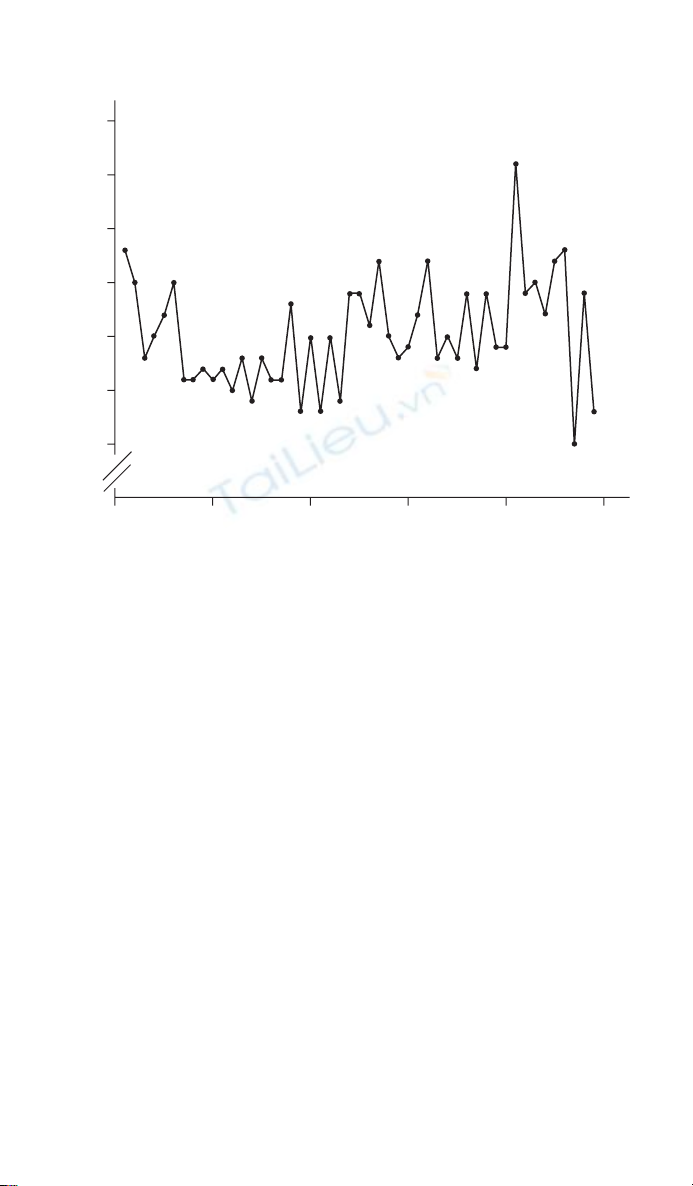
An example of a time series plot is given in Figure 8.1. The data are the
number of infant deaths per day in England and Wales over a 7-week period
during 1979.1 The important points to consider when drawing a time series
are that time should be on the X-axis (horizontal) and the series of events
that are being monitored, the observations, are on the Y-axis (vertical). In
addition, adjacent points should be joined by straight lines. If the origin has
been omitted this should be made clear, as here, by two diagonal lines on the
axis line. Care should be taken when examining published time series plots.
They are often used in newspapers and a common trick is not to show the
origin, so that a small trend can appear magnifi ed. This is discussed in more
detail in Section 2.3.
Time series plots and survival curves 91
8.3 Lowess smoothing plots
Lowess smoothing plots are a useful way of displaying some time series
data.2 They are described in more detail in Section 5.3, where they are
applied to continuous data. For time series they are useful for investigating
non-linear trends, as demonstrated here. Figure 8.2a shows the number of
prescriptions for non-selective serotonin reuptake inhibitors (SSRIs), a type
of antidepressant, over a 3.5-year period, from 2002 to 2006 for one general
practice in Yorkshire, England (Senior J., Personal Communication, 2006).
The scatter plot seems to show a generally increasing trend, with more scatter
towards the end. However, fi tting a lowess smoothing curve with bandwidth
of 50% suggests that in fact the number of prescriptions peaked at around
month 30 (Figure 8.2b). This corresponds to the time when national guide-
lines were published by NICE recommending that SSRIs should be prescribed
in preference to non-SSRIs for the treatment of depression. The peak is sug-
gested by the data, and so lowess plots are useful for data exploration, but not
for testing hypotheses. Note that as the Y-axis does not begin at the origin
(value 0) this has been indicated by two parallel lines.
45
40
35
30
25
20
15
0102030
Time (days)
Infant deaths (n)
40 50
Figure 8.1 Daily infant deaths in England and Wales over a 7-week period during
1979.1
![Tài liệu Nhập môn khoa học dữ liệu [Chuẩn nhất]](https://cdn.tailieu.vn/images/document/thumbnail/2026/20260401/baobinh_011/135x160/57531775122890.jpg)


![Tổng quan về Physique: Giới thiệu chung [chuẩn nhất]](https://cdn.tailieu.vn/images/document/thumbnail/2012/20120719/suthebeo/135x160/1214236_349.jpg)


![Phân tích số liệu và biểu đồ bằng R: Tài liệu [Mô tả/Hướng dẫn/Kinh nghiệm chi tiết]](https://cdn.tailieu.vn/images/document/thumbnail/2026/20260430/ntu.danghuy@gmail.com/135x160/46211777946371.jpg)

