
REGULAR ARTICLE
Potential sources of uncertainties in nuclear reaction modeling
Stephane Hilaire
1,*
, Eric Bauge
1
, Pierre Chau Huu-Tai
1
, Marc Dupuis
1
, Sophie Péru
1
, Olivier Roig
1
,
Pascal Romain
1
, and Stephane Goriely
2
1
CEA, DAM, DIF, 91297 Arpajon, France
2
Institut d’Astronomie et d’Astrophysique, Université Libre de Bruxelles, CP-226, 1050 Brussels, Belgium
Received: 31 October 2017 / Received in final form: 12 February 2018 / Accepted: 4 May 2018
Abstract. Nowadays, reliance on nuclear models to interpolate or extrapolate between experimental data
points is very common, for nuclear data evaluation. It is also well known that the knowledge of nuclear reaction
mechanisms is at best approximate, and that their modeling relies on many parameters which do not have a
precise physical meaning outside of their specific implementations in nuclear model codes: they carry both
specific physical information, and effective information that is related to the deficiencies of the model itself.
Therefore, to improve the uncertainties associated with evaluated nuclear data, the models themselves must be
refined so that their parameters can be rigorously derived from theory. Examples of such a process will be given
for a wide sample of models like: detailed theory of compound nucleus decay through multiple nucleon or gamma
emission, or refinements to the width fluctuation factor of the Hauser-Feshbach model. All these examples will
illustrate the reduction in the effective components of nuclear model parameters, through the reduced dynamics
of parameter adjustment needed to account for experimental data. The significant progress, recently achieved
for the non-fission channels, also highlights the difficult path ahead to improve our quantitative understanding of
fission in a similar way: by relying on microscopic theory.
1 Introduction
The modeling of nuclear reactions involves several models
connected with each other to produce nuclear data. Three
main models (Fig. 1) are usually employed in modern
nuclear reaction codes such as TALYS [1] or EMPIRE [2]:
the optical model, the pre-equilibrium model and the
compound nucleus model. All these models rely on a large
number of inputs as well as on more or less valid
approximations. Even though it is possible nowadays to
reproduce, with a rather good accuracy, available experi-
mental data by adjusting the various parameters driving
the nuclear reaction models, several approximations are
still known to be compensated by these parameter
adjustment and/or by an interplay between the models
themselves. It is therefore important, to improve our
understanding of the physical processes occuring during a
nuclear reaction as well as the predictive power of the
modeling itself, to be able to reduce the sources of error
compensation by suppressing some of the approximations
known to play a role or by improving the modeling of
specific inputs required by nuclear models. In this paper, we
illustrate some important issues which we think should be
carefully accounted for to reduce potential sources of
uncertainties in the evaluation process. Section 2 discusses
the optical model which has to be as accurate as possible.
Indeed, since this model is at the basis of the evaluation
process, any error or inaccuracy it yields has an impact on
both the pre-equilibrium and the compound nucleus model
which must then be tuned to compensate the possible
deficiencies of the optical model. Section 3 focuses on the
differences that can be obtained depending upon whether
one uses a classical pre-equilibrium model or a more
microscopic approach to populate the compound nucleus
before it decays. Section 4 illustrates few other sources of
uncertainties such as those related to the fission channel,
the width fluctuation correction factor (WFCF) or the
gamma-ray strength functions, required as inputs to the
compound nucleus model. Conclusions and prospects are
finally drawn in Section 5.
2 The optical model
As illustrated in Figure 1, the optical model is the first
model used in the nuclear reaction modeling. This model
enables to separate the incident projectile flux into three
main components: the shape elastic, the direct inelastic
and the reaction cross-sections. It also provides transmis-
sion coefficients for light particles whose emission is treated
within the compound nucleus model framework. As a
*e-mail: stephane.hilaire@cea.fr
EPJ Nuclear Sci. Technol. 4, 16 (2018)
©S. Hilaire et al., published by EDP Sciences, 2018
https://doi.org/10.1051/epjn/2018014
Nuclear
Sciences
& Technologies
Available online at:
https://www.epj-n.org
This is an Open Access article distributed under the terms of the Creative Commons Attribution License (http://creativecommons.org/licenses/by/4.0),
which permits unrestricted use, distribution, and reproduction in any medium, provided the original work is properly cited.
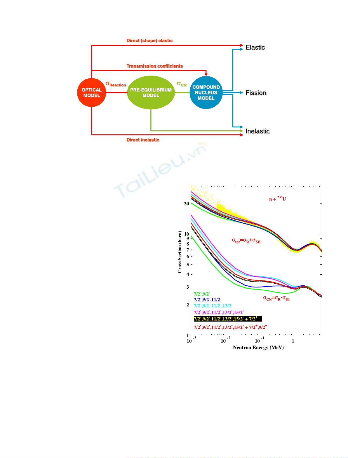
consequence, any error or inaccuracy introduced at this
level of the modeling process will directly influence the
following steps, namely the pre-equilibrium and the
compound nucleus models. Several approaches are avail-
able to construct an optical model potential. Microscopic
methods aiming at producing an Optical Model Potential
(OMP) [3–6] based on nucleon–nucleon interactions are
not yet usable for evaluation purposes due to their lack of
accuracy or to a too narrow range of application. Therefore
phenomenological [7–9] or semi-microscopic approaches
[10–12] are usually employed for applications.
When many experimental data are available, phenom-
enological approaches are clearly prefered since the number
of parameters on which they rely provide with a high degree
of flexibility and the possibility to obtain very accurate fits
of measured data. However, the price to pay is then an in
depth analysis of the sensitivity of the output to the input
parameters. In the case of a deformed target, beyond the
OMP parameters, the adopted coupling scheme as well as
the deformation parameters also play a crucial role. A
typical illustration of the impact of the number of inelastic
levels introduced in coupled channel (CC) methods is
shown in Figure 2. As can be observed, the total cross-
sections reaches rather similar values, at least compatible
with experimental data within error bars, for various
choices of the number of coupled levels while the compound
nucleus formation cross-section remains much more
sensitive to the choice of the coupling scheme. With such
differences, the other channels predictions, in particular
the fission cross-section, will be clearly influenced by the
number of coupled levels considered, meaning that
uncertainties in the fission channel do not only depend
on the sole uncertainties on fission model parameters, as it
might be thought at first glance.
In the case of the so-called Jeukenne-Lejeune-Mahaux
(JLM) semi-microscopic[10–12] approach, one does not have
the freedom to fit cross-section as for the phenomenological
OMP. Indeed, the free parameters of the approach have been
fixed on a selected set of nuclei and are not modified when
changing the target. The only freedom is then linked to the
structure description of the target. For a 28 MeV (p,p0)
reaction on
36
S for instance (Fig. 3), it can be observed that
describing the target nucleus within the quasiparticle
random phase approximation (QRPA) framework [13,14]
Fig. 1. Flowchart of the sequence of models required to describe a nuclear reaction. The optical model enables to separate the incident
flux (total cross-section) in three separate contributions (the shape elastic, the reaction and the direct inelastic cross-sections) and
provides the compound nucleus with light particles transmission coefficients. Part of the reaction cross-section (s
Reaction
) is then
processed with the pre-equilibrium model to feed inelastic channels as well as the compound nucleus model with the remaining flux
(s
CN
). s
CN
is then spread over all outgoing channels by the compound nucleus model.
Fig. 2. Total (s
tot
) and compound nucleus formation (s
CN
)
cross-sections obtained increasing the number of coupled levels
in the coupled channel approach for neutron induced reaction
on
235
U.
2 S. Hilaire et al.: EPJ Nuclear Sci. Technol. 4, 16 (2018)
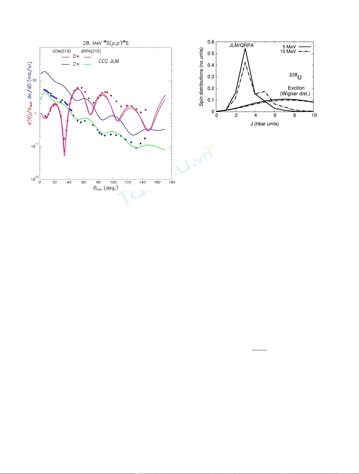
enables to reproduce available experimental data for
inelastic scattering off the 2
+
level better than when the
five-dimensional collective hamiltonian (noted GCM for
Generator Coordinate Method in Fig. 3) approach [15]is
used, while the elastic scattering is almost not modified.
3 The pre-equilibrium model
Another feature which is known to impact the cross-section
determination for various reactions is related to the
modeling of the pre-equilibrium emission mechanism for
which one or several particles are emitted before a
compound nucleus is formed. In many applications, pre-
equilibrium is described within the phenomenological
exciton model which is semi-classical and contains
parameters tuned on a relevant set of (n,xn) and (p,xp)
observables. An alternative method, recently developed
[16,17], employs the QRPA nuclear structure model [13,14]
in a relevant microscopic reaction approach, the JLM
folding model, to determine the fast excitation mechanism
of the target nuclei which occurs during the pre-equilibrium
process. Depending upon the method employed, the
compound nucleus population after such direct-like
interaction, is strongly modified. This is illustrated in
Figure 4 for a
238
U(n,n0g) reaction. After the pre-
equilibrium emission of a neutron, the formed compound
nucleus has a spin population which peaks at much lower
values when a microscopic approach is used and the spin
distribution structure does not follow the statistical
Wigner distribution associated to the exciton model.
This aspect strongly impacts the determination of
gamma-ray emission cross-sections for transitions between
discrete states of the residual nucleus. Indeed, if the
compound nucleus is formed with mainly low spin, the
system will have to go through many transitions to reach a
high spin. Thus g-emission from states with high spin will
be strongly hindered. Figure 5 illustrates this aspect as it
shows that calculations based on the exciton model and the
Wigner spin distribution over-predict (n,n0g) transition
from the 10
+
state while the QRPA-based approach
provides a magnitude in agreement with the measured
values.
It would be possible to mimic the QRPA-based spin
distribution adjusting the Wigner spin distribution
parameters but such an effectiveness would clearly hide
a misunderstanding of the physics in order to fit the
observed transition.
4 The compound nucleus model
The compound nucleus model is the last model involved in
the evaluation of nuclear reaction. This model, based on the
statistical Hauser-Feshbach approach, provides the cross-
section between an incident channel aand an outgoing
channel bas
sab ¼TaTb
PcTc
Wab:ð1Þ
In equation (1),T
a
and T
b
correspond to the incident and
outgoing transmission coefficients, the sum P
c
T
c
runs over
all open channels and W
ab
is the WFCF accounting for the
fact that the entrance and outgoing channel are not totally
independent [21]. It has been recently demonstrated
[22–24] that, for well deformed nuclei, the usually neglected
Engelbrecht-Weidenmüller transformation (EWT) [25],
known to be required for a rigourous description of the
WFCF was playing a rather important role. More
precisely, whereas it was thought that the WFCF only
enhances the elastic channel and decreases all inelastic
channel, it has been shown that for inelastic levels strongly
Fig. 3. (p,p0) angular distribution on
36
S for the ground state and
first 2
+
state using two microscopic structure approaches (GCM
or QRPA see text for details) to determine transition densities
required for a coupled channel calculation within the semi-
microscopic JLM approach.
Fig. 4. Compound nucleus spin distribution of the
238
U
compound nucleus formed after a fast neutron emission. The
Wigner distribution associated to the exciton model is compared
to the QRPA-based approach of references [16,17].
S. Hilaire et al.: EPJ Nuclear Sci. Technol. 4, 16 (2018) 3
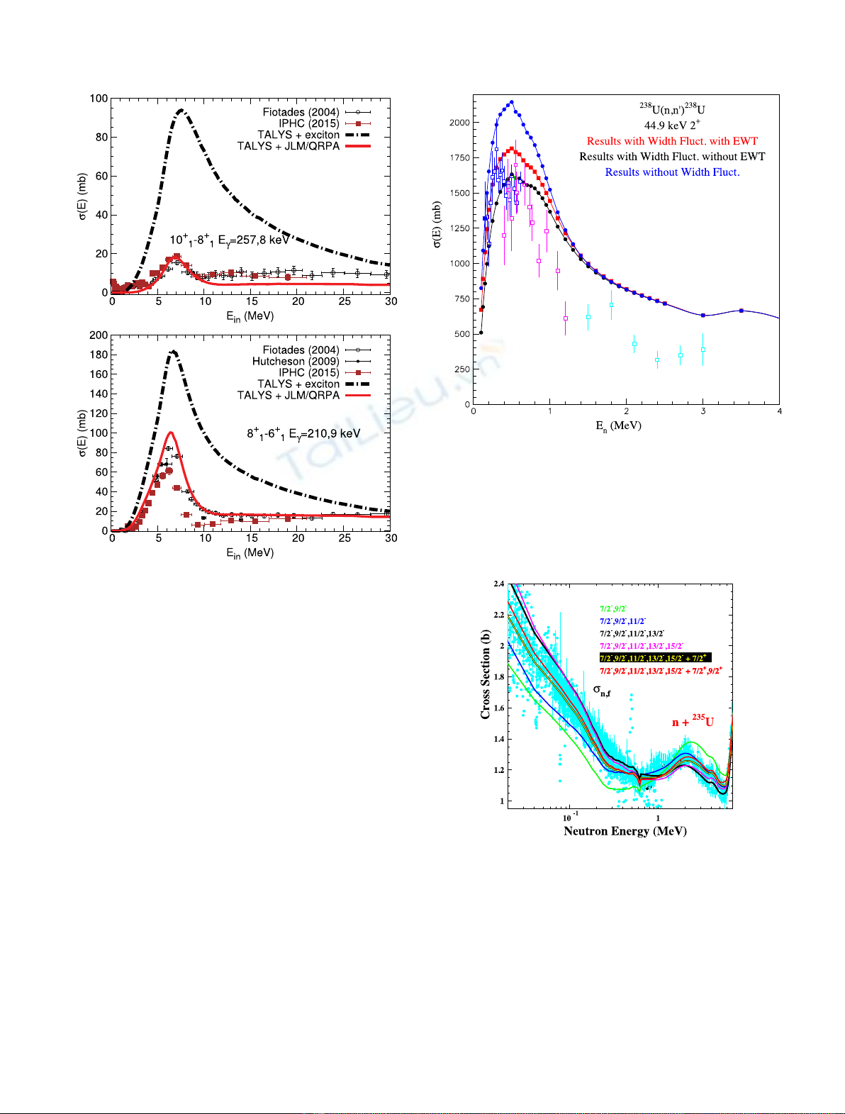
coupled to the ground state, an enhancement of the
inelastic cross-section was also observed. This effect is
illustrated in Figure 6 where a comparison is shown
between various predictions and the direct inelastic cross-
section off the first 2
+
level in
238
U.
One can understand that if the EWT is accounted for,
the adjustment of the OMP parameters enabling to fit
available experimental data will not be the same as if one
does not account for the EWT, unless the energy region
where the EWT plays a role is not used to constrain the
OMP parameters. It is thus clear that if the EWT effects
are hidden in the parameters entering the definition of the
OMP, avoidable error compensations are introduced in the
evaluation.
Another example of compensation effect is also
illustrated in Figure 7. In this case, one can study the
impact of the coupling scheme considered in the CC-OMP
when looking at the corresponding fission cross-sections.
Depending on the number of coupled levels introduced, the
fission cross-section varies significantly, reflecting, as
shown in Figure 2, the way the number of coupled level
modifies the compound nucleus formation cross-section.
One could of course improve, for each choice of the coupling
scheme, the fit of the fission cross-section by fine tuning the
fission model parameters. This would however mean that
the fission model would counterbalance a restricted
coupling scheme in the CC approach.
The gamma emission is also a nice illustration of
compensation effects. Within the Brink-Axel hypothesis
[27,28], the gamma transmission coefficient reads
TXℓEg¼2pfXℓEgE2ℓþ1
g;ð2Þ
Fig. 5.
238
U(n,n0g) cross-sections for two transitions in the
ground state rotational band (see details on plots). Two Talys
calculations, which used the exciton (dashed black curves) or the
JLM/QRPA model (full red curves) for pre-equilibrium, are
compared to experimental data (symbols) [18–20].
Fig. 6. Inelastic cross-section off the first 2
+
level of
238
Uas
function of the excitation energy E
n
. The red (resp. black) line
shows the theoretical prediction obtained using (resp ignoring)
the EWT with the Soukhovitski
~
ioptical model potential [26]. The
blue line shows the predictions obtained ignoring width
fluctuation corrections. Experimental data are taken from the
EXFOR database [29].
Fig. 7. Fission cross-section obtained increasing the number of
coupled levels in the CC approach for neutron induced reaction on
235
U.
4 S. Hilaire et al.: EPJ Nuclear Sci. Technol. 4, 16 (2018)
where E
g
is the energy of the emitted gamma of type X
(X=Eor Mfor electric or magnetic transitions) and
multipolarity ℓ, and where f
Xℓ
(E
g
) is the energy dependent
gamma-ray strength function whose analytical expression
follows a Lorentzian shape. For thermal neutrons, the
compound nucleus excitation energy corresponds to the
neutron separation energy S
n
and the average radiative
with G
g
is entirely due to s-wave neutrons, so that the
gamma-ray strength function satisfies the following
equation
2pGg
D0
¼GnormX
JP
X
Xℓ
X
I0Jþℓ
I0Jℓ
X
P0
∫Sn
0TXℓEgrSn
EgI0p0dXℓP0dEg:ð3Þ
In this equation, the J,Psum runs over the compound
nucleus states with spin Jand parity Pthat can be formed
with s-wave incident neutrons and I
0
,P
0
denote the spin
and parity of the final states to which a photon of type X
with multipolarity ℓcan be emitted. The multipole
selection rules are d(X=E,ℓ,P
0
)=1 if P=(1)
ℓ
P
0
for
Electric transition, d(X=M,ℓ,P
0
)=1 if P=(1)
ℓ+1
P
0
for magnetic transitions and d(X,ℓ,P
0
) = 0 otherwise.
Finally, ris the compound nucleus nuclear level density
and D
0
the average spacing of s-wave resonances. In
practice, whereas G
norm
should be equal to unity, one often
has to use a different value for G
norm
to ensure equation (3)
is verified. Hence, the gamma transmission coefficient is
multiplied by an arbitrary normalization factor G
norm
,
which is compensating for the level density option that can
be chosen when modeling a nuclear reaction and/or for
deficiencies of the chosen gamma strength function. An
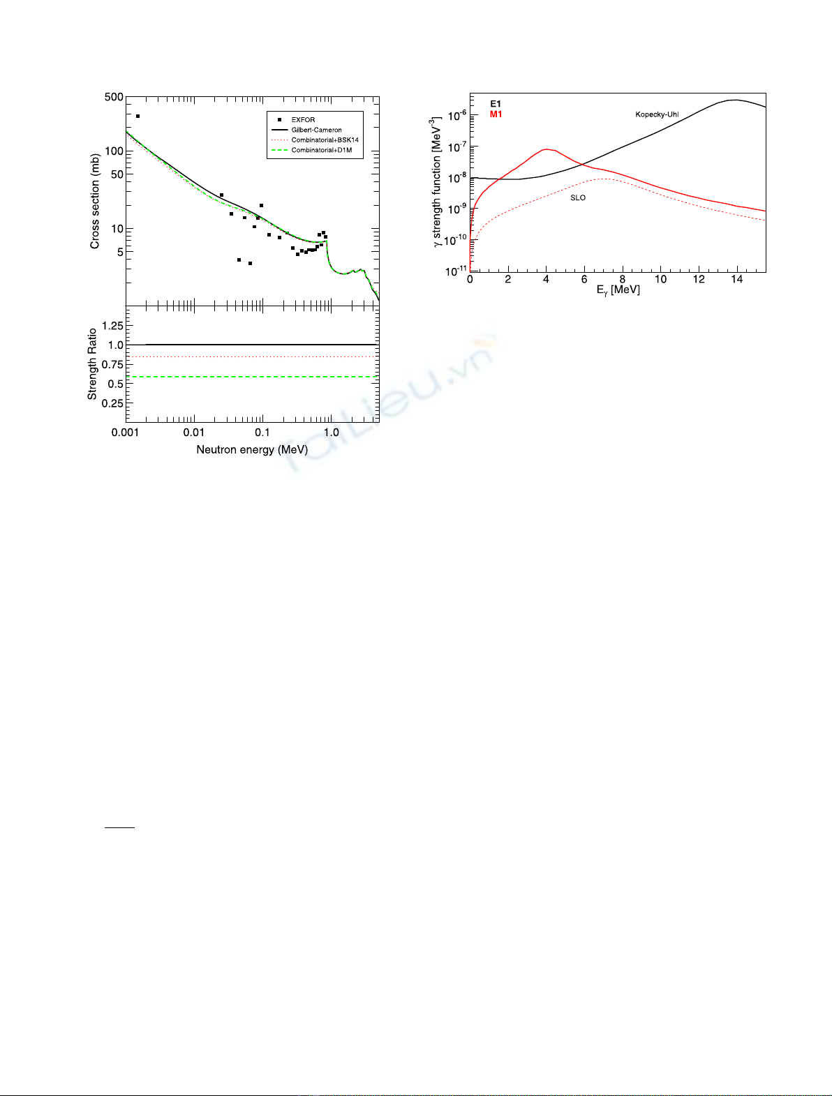
illustration of this compensation is given in Figure 8.
In this figure, the
56
Fe neutron capture is shown using
various level density models for the
57
Fe compound
nucleus keeping the same gamma-ray strength function
expressions (Kopecky and Uhl [33] for E1 and Standard
Lorentzian [27,28] otherwise). Thanks to the normaliza-
tion of equation (3), one can observe that very similar
cross-section predictions are obtained. However, the
corresponding gamma-ray strength functions are strongly
modified by the normalizations depending on the level
density option. It is therefore clear that if the normaliza-
tion procedure of equation (3) enables to reproduce
capture cross-sections data, photoabsorption cross-sec-
tion will not be always reproduced.
A more refined approach has been recently studied to
solve such an inconsitency. It consists in introducing an
arbitrary low energy extra gamma-ray strength con-
strained to simultaneously describe capture and photo-
absorption data [37–39]. The justification for such an extra
strength stems from the fact that several experiment have
reported, for low gamma-ray energies, strengths which are
higher than the usually adopted analytical expression that
have been adjusted to reproduce experimental data at
energies above the region where such disagreement are
observed. In this case, one can obtain G
norm
values which
are closer to unity by enhancing locally the gamma-ray
strength without modifying the high energy agreement
with photoabsorption data. This procedure is illustrated in
Figure 9 for the
177
Lu E1 and M1 strengths.
Fig. 8. Top panel:
56
Fe(n,g)
57
Fe cross-section as function of the
neutron incident energy. The black squares correspond to
EXFOR data [29], the full black line is the prediction obtained
using the default level density model implemented in the TALYS
code [1,30], the red dotted line using the combinatorial level
density model of reference [31] and the green dashed line the
combinatorial level density model of reference [32]. Bottom panel :
ratio between the strength functions obtained after the normal-
ization deduced from equation (3) is applied and the strength
function corresponding to the default level density option.
Fig. 9. E1 and M1 strength function of
177
Lu. The full black line
shows the so-called Kopecky and Uhl [33] model implemented in
TALYS for the E1 strength. The dashed red line corresponds to
the default model for the M1 strength, namely the standard
Lorentzian model [27,28]. The full red line shows the M1 strength
obtained introducing a supplementary component in the M1
strength with a second Lorentzian centered around 4 MeV.
S. Hilaire et al.: EPJ Nuclear Sci. Technol. 4, 16 (2018) 5


![Ngân hàng trắc nghiệm Kỹ thuật lạnh ứng dụng: Đề cương [chuẩn nhất]](https://cdn.tailieu.vn/images/document/thumbnail/2025/20251007/kimphuong1001/135x160/25391759827353.jpg)