
REGULAR ARTICLE
A methodology for performing sensitivity analysis in dynamic fuel
cycle simulation studies applied to a PWR fleet simulated
with the CLASS tool
Nicolas Thiollière
1,*
, Jean-Baptiste Clavel
2
, Fanny Courtin
1
, Xavier Doligez
3
, Marc Ernoult
3
, Zakari Issoufou
3
,
Guillaume Krivtchik
4
, Baptiste Leniau
1
, Baptiste Mouginot
5
, Adrien Bidaud
6
, Sylvain David
3
, Victor Lebrin
1
,
Carole Perigois
1
, Yann Richet
2
, and Alice Somaini
3
1
Subatech, IMTA-IN2P3/CNRS-Université, 44307 Nantes, France
2
IRSN/PSN-EXP/SNC/LNC, BP 17, 92262 Fontenay-aux-Roses, France
3
Institut de Physique Nucléaire d’Orsay, CNRS-IN2P3/Univ. Paris-Sud, Orsay, France
4
CEA, DEN, Cadarache, DER, SPRC/LECY, 13108 Saint-Paul-lez-Durance, France
5
Univ. of Wisconsin Madison, Department of Nuclear Engineering and Engineering Physics, Madison, WI, USA
6
Laboratoire de Physique Subatomique et de Cosmologie, Université Grenoble-Alpes, CNRS/IN2P3, Grenoble, France
Received: 23 August 2017 / Received in final form: 15 January 2018 / Accepted: 3 April 2018
Abstract. Fuel cycle simulators are used worldwide to provide scientific assessment to fuel cycle future
strategies. Those tools help understanding the fuel cycle physics and determining the most impacting drivers at
the cycle scale. A standard scenario calculation is usually based on a set of operational assumptions, such as
reactor Burn-Up, deployment history, cooling time, etc. Scenario output is then the evolution of isotopes mass in
the facilities that composes the nuclear fleet. The increase of computing capacities and the use of neutron data
fast predictors provide new opportunities in nuclear scenario studies. Indeed, a very high number of calculations
is possible, which allows testing a high number of operational assumptions combinations. The global sensitivity
analysis (GSA) formalism is specifically well adapted for this kind of problem. In this new framework, a scenario
study is based on the sampling of operational data, which become input variables. A first result of a scenario
study is the highlight of relations between operational input data and outputs. Input variable subspace that
satisfy optimization criteria on an output, such as plutonium incineration or stabilization, can also be
determined. In this paper, a focus is made on the methodology based on GSA. This innovative methodology is
presented and applied to a simple fleet simulation composed of a PWR-UOx fuel and a PWR-MOx fuel.
Calculations are done with the fuel cycle simulator CLASS developed by the CNRS/IN2P3 in collaboration with
IRSN. The design of experiment is built from five fuel cycle input sampled variables. Sensitivity indices have
been calculated on plutonium and minor actinide (MA) production. It shows that the PWR-UOx Burn-Up and
the fraction of PWR-MOx fuel are the most important input variables that explain the plutonium production.
For the MA production, main drivers depend strongly on isotopes. Sensitivity analysis also reveals input variable
subspace responsible of simulation crash, what led to an important improvement of the model algorithms. An
equilibrium condition on the plutonium mass in the stockpile used for building MOx fuel has been applied. The
solution is represented as a subspace in the PWR-UOx Burn-Up and PWR-MOx fraction input space. For
instance, achieving a plutonium equilibrium in a stockpile fed by a PWR-UOx that operates at 40 GWd/t
requires a PWR-MOx fraction between 9 and 14%. This study also provides data related to plutonium
incineration induced by the utilization of the MOx.
1 Introduction and motivations
Fuel cycle simulators associated to innovative analysis
methodologies are developed for enhancing the scientific
knowledge on nuclear fuel cycle physics. By calculating
radioactive inventory evolution in each unit of an evolving
fuel cycle, dynamic fuel cycle tools help understanding fuel
cycle physics highlighting the drivers for each specific
output observable. Also, an electro-nuclear fuel cycle
scenario study is connected to other energy and electricity
production sources. Many scientificfields may be involved,
such as economy, sociology, etc. Fuel cycle simulators are
*e-mail: nicolas.thiolliere@subatech.in2p3.fr
EPJ Nuclear Sci. Technol. 4, 13 (2018)
©N. Thiollière et al., published by EDP Sciences, 2018
https://doi.org/10.1051/epjn/2018009
Nuclear
Sciences
& Technologies
Available online at:
https://www.epj-n.org
This is an Open Access article distributed under the terms of the Creative Commons Attribution License (http://creativecommons.org/licenses/by/4.0),
which permits unrestricted use, distribution, and reproduction in any medium, provided the original work is properly cited.

then useful tools for building interdisciplinary researches in
link with scientificfields mentioned above. As a conse-
quence, technical and interdisciplinary researches on fuel
cycle produce analysis that could help enlighten the debate
and the decision making process in the context of the
energy transition.
A lot of different fuel cycle simulation tools are
developed by nuclear engineering and research institutions.
Several level of detail are reached by available tools, from
the simple spreadsheet to a complex code. This complexity
depends on the reactor type or fuel characteristics. For
innovative reactors, such as GEN IV reactors, as for
reprocessed fuel such as advanced MOx fuel, a high level of
reactor physics is required to ensure a high level of
confidence in results. Nuclear energy policy is usually part
of a national strategy. This is why a lot of scenario studies
based on nuclear fuel cycle simulators are focused on the
country scale, taking into account the country specificities
[1–3]. Nevertheless, some dedicated studies could be also
extended to continent in the case of high relationship level
between countries, as Europe for instance [4].
In France, the most advanced software for fuel cycle
simulations is the code COSI [5], developed by CEA
1
. The
physics is represented with a very high level of detail. At
the international level, a lot of tools are available. For
instance, the agent-based nuclear fuel cycle simulation
Cyclus [6] is developed and used for a large range of
applications: non-proliferation [7], nuclear archeology [8],
etc. The code VISION [9] developed by DOE laboratories is
used in the framework of the system analysis working group
of the United States research program on advanced fuel
cycles. We can also mention the code EVOLCODE [10]
developed by the CIEMAT
2
, the code DANESS (Dynamic
Analysis of Nuclear Energy System Strategies) [11]
developed by the international operating expert firm
Nuclear21, and many others.
A lot of work has already been produced on input
variables uncertainty propagation. The nuclear data uncer-
tainty propagation in nuclear fuel cycle simulation outputs
has been assessed [12]. The Nuclear Energy Agency Expert
Group on Advanced Fuel Cycle Scenarios has produced a
study to evaluate the effects of the uncertainties of input
parameters on the outputs of fuel cycle calculations [13].
The present paper represents a continuation of the
effort described below. The main innovation is the
definition of a complete design of experiment that leads
to a relative high number of fuel cycle simulations. In this
representation, input parameters are not considered as
uncertainties, but as scenario study results that fit with
selection criteria imposed on outputs.
Usually, nuclear fuel cycle scenario studies are based on
few very detailed simulations. Reactors and other fuel
facilities parameters are defined by the user. Reactors could
be defined by the thermal power, the specific power and the
discharge Burn-Up. The physics related to the reactor
depends on the characteristics of the core such as geometry,
composition and temperature. Mean cross sections needed
for solving the evolution equations are processed from the
neutron spectrum. A new technology deployment plan is
defined by the deployment date and the deployment
kinetic, usually optimized from several upstream calcu-
lations. Input variables are called scenario assumptions and
their choice strongly impacts the output analyses and then,
the scenario evaluation.
The last generation of fuel cycle simulation tools has
been developed in order to be fast. The codes processing
speed as well as the increase of the computing capacities
open a new paradigm for fuel cycle simulator utilization,
since a very high number of calculations could be
achievable.
The present work shows how to build and assess a
simple nuclear scenario, from tools provided by the
sensitivity analysis. The method supposes to build a
design of experiment in which input variables are sampled.
Sensibility indices are used to select the most impactive
variables on an specific output which helps to guide the
analysis. The effect of input variables on model outputs
could be determined and quantified. Finally, this method-
ology provides also solution spaces from any criteria on
output observable. The paper presents also an illustration
of the method with an adapted design of experiment used to
study a simplified PWR-UOx MOx fuel fleet. The focus is
made here on the methodology precise description, and on
some relevant results.
The GSA is described and its contribution on fuel cycle
studies is highlighted. Then, the fuel cycle simulator
CLASS, used as the fuel cycle model for the sensitivity
analysis study performed on a simplified PWR UOx and
PWR MOx fleet is presented. This methodology can be
used on any fuel cycle strategy evaluation. The design of
experiment is described, as the methodology for storing and
analyzing output data. Finally, input variables impact on
plutonium and minor actinides (MA) production will be
presented.
2 Global sensitivity analysis for fuel cycle
studies
This section aims to describe the framework of the fuel
cycle simulations used to build the analysis study of a
simplified PWR-UOx MOx fleet. The current methodology
used for building scenario studies is explained and the
global sensitivity analysis (GSA) innovative contribution
is detailed.
2.1 Dynamic fuel cycle studies
A fuel cycle simulation is usually based on a complex
computer code that models material irradiation in reactors,
cooling phases and exchanges in facilities. Most important
effort concerns, in the neutron physics point of view, the
fresh fuel composition needed to reach reactor require-
ments and the calculation of the composition according to
the irradiation conditions.
The fresh fuel determination is usually based on a fuel
loading model (FLM) that aims to provide fractions of
materials needed to satisfy reactor requirements (maximal
1
Commissariat à l’énergie atomique et aux énergies alternatives.
2
Centro de Investigaciones Energèticas, Medioambientales y
Tecnològicas.
2 N. Thiollière et al.: EPJ Nuclear Sci. Technol. 4, 13 (2018)

Burn-Up, regeneration rate, etc.) for any available
materials. This could be achieved for instance by a simple
formula, by the use of
239
Pu equivalent methods [14]or
with neural network based predictors [15]. An additional
algorithm is then needed to determine the appropriate
composition built from available stocks.
Once the fresh fuel is built, the model calculates the
evolution of materials under neutron irradiation. The
calculation scheme is based on the resolution of the two
following equations:
–the Boltzmann equation provides the neutron spectrum
which leads to the mean cross sections calculation;
–the Bateman equations are the isotopic vector evolution
equations solved from initial composition and specific
thermal power.
In practice, the coupling between those two equations
leads to precise calculated inventory. Indeed, when the
composition is evolving, neutron spectrum has to be
frequently updated in order to use correct mean cross
sections. To precisely simulate fuel evolution in a fuel cycle
simulator, two methods are usually used. The first one
consists to build a coupling with a neutron transport code
which includes also a Bateman equations solver. This
solution is very accurate but requires a high computing
time. The second solution consists in building and using
neutron data predictors in the fuel cycle simulation. The
advantages of predictors is that computing time is very fast
compared to neutron code coupling. Nevertheless, a
minimum bias in comparison with the reference calculation
must be guaranteed.
A fuel cycle simulator integrates several spatial and
temporal scales connected to different physics phenomena:
–nuclear reactions induced by neutrons flux;
–nuclear core isotopic composition evolution under the
neutron flux;
–nuclear fleet transition induced by reactor deployment or
phase out;
–middle and long term inventory activity decay.
As a consequence, a dynamic fuel cycle simulation
output may be characterized by a high uncertainty, with
several origins that could be classified as follow:
–nuclear data used to calculate neutron flux and mean
cross sections;
–reactors (resp. cycle) simplifications in the transport
(resp. fuel cycle) simulations;
–operational assumptions imposed in the fuel cycle
simulation.
The nuclear data include microscopic cross sections,
fission and decay data used in the transport code. Effect of
nuclear data uncertainties on a fuel cycle output has been
investigated in [12]. Reactor simulation simplifications are
coming from the difficulties to simulate precisely a full core
reactors taking into account all the specificities (irradiation
history, reactivity control with boron or control rods, fuel
loading patterns, etc.). The common methodology for fuel
cycle simulations consists in using assemblies with mirror
conditions, which leads to increase uncertainty. The
impact of using assembly calculation has been investigated
in [16]. Fuel cycle simplifications could be part of the model
or decided by the user during the scenario construction.
Among them, we can point for instance first loadings after
reactor operation starting date, shutdown of unit duration
during fresh fuel loadings, etc. The impact of those kind of
simplifications should be quantified in the future.
Operational assumptions are operational data that are
user-defined in a fuel cycle simulation. That could be
reactor Burn-Up, thermal power, loading factor, deploy-
ment date or other facility characteristics. Those kind of
data could not be determined since fuel cycle simulators
aims to model future trajectories. The utilization of
neutron data predictors and the increase of computing
capacities provide new opportunities to perform nuclear
scenario studies since a very high number of calculations is
currently reachable. In this new vision, operational
assumptions are not unknown data but become scenario
results obtained by applying optimization criteria on
scenario outputs. In a longer-term perspective, this
methodology based on a multi-criteria analysis that would
take into account technical, economical and even sociolog-
ical criteria could be considered.
Massive fuel cycle simulation requires a suitable
mathematical framework and GSA fulfills perfectly this
role.
2.2 Global sensitivity analysis (GSA)
GSA is used in many research fields involving modeling of
complex physical phenomena. Each field applies GSA
according to its specific needs. A lot of relevant bibliographi-
cal sources are available, for instance [17–19]. According
to [20], GSA provides relevant answers for following
applications:
–test if the model is in agreement with the simulated
process;
–determine most impacting input variables on an output
observable variability;
–highlight negligible input variables or model parameters;
–highlight and understand interactions between variables.
For fuel cycle simulators applications, GSA could also
help understanding the physics from input and output
variables relations highlight. In addition, it could provide
relevant informations for detecting and correcting errors in
the code algorithms.
For application involving a lot of variables with
potential interactions, variance based methods are power-
ful and suitable tools. A lot of sensitivity indices may be
used. Since fuel cycle studies have a high input data
number and spread, output observables (such as plutonium
mass at a given time) may have a high variability. Sobol’
indices are efficient estimators of input variables or model
parameters weight in an output variability and have been
chosen in the framework of the proposed application (see
Sect. 4.2).
2.3 Design of experiment
The fuel cycle simulation used to illustrate the methodolo-
gy describes a simplified nuclear fleet composed by PWR
loaded with uranium oxide (UOx) and mixed oxide (MOx)
N. Thiollière et al.: EPJ Nuclear Sci. Technol. 4, 13 (2018) 3
fuels. Since the goal of the work is to study impact of
reactor parameters on fuel cycle simulation outputs, one
reactor of each type (UOx and MOx) is defined. It has been
shown [1] that this kind of simplifications produced results
that could be extrapolated to complex fleet simulation with
reasonable accuracy. The MOx fuel integration impact will
also be assessed by sampling the PWR-MOx fraction. Total
thermal power at beginning of scenario is 2.1 GW
th
(2.8 GW
th
with a load factor of 0.75) and total heavy
nuclei mass is 72.3 tons. During the calculation, reactors
power and mass can be modified but the specific thermal
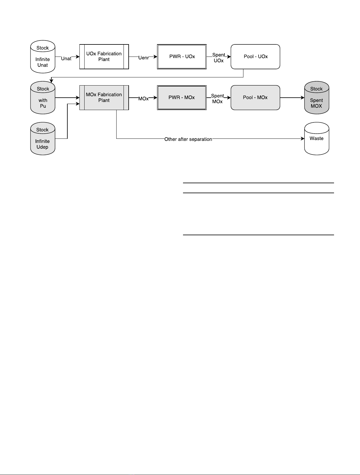
power remains constant. Simulations schematic represen-
tation is shown in Figure 1.
An infinite stock feeds with natural uranium a
fabrication plant that provides enriched uranium to the
PWR-UOx reactor. Uranium enrichment is calculated
from reactor required Burn-Up. An irradiation cycle is
done and the spent UOx fuel is sent to the pool. After a
cooling time defined by the user, the spent fuel is sent to a
stock that is used by the MOx fabrication plant to build
PWR-MOx fresh fuel. The fabrication plant separates the
plutonium needed and add depleted uranium. During the
separation process, the reprocessing losses are 0. The
plutonium fraction in the MOx fuel is calculated to satisfy
the required Burn-Up. The MOx fuel is irradiated in the
reactor and sent to a pool and a stock after the cooling time.
The power of the fleet is supposed to be constant during the
scenario that end after 100 years of operation. Neverthe-
less, this condition can not always be realized because of the
availability of the plutonium, as discussed in Section 4.3.In
practice to simplify calculations, reactors lifetime has been
set at the duration of the scenario. If this is not realistic
from the technical point of view and if we could have
defined more reactors, this has no impact on the inventory
evolution calculation. Between t= 0 and t= 20 years, one
PWR-UOx is operated and the plutonium builds-up in the
stockpile. At t= 20 years until the end of the scenario at
t= 100 years, a fraction of the total power is distributed to
a PWR-MOx reactor.
Simulations were done with the fuel cycle simulator
CLASS, described in Section 3. A set of five input variables
of the fuel cycle simulation has been selected. Each input
data has been uniformly sampled between a minimum and
a maximum value that seems reasonable according to
technological knowledge. Table 1 presents sampled input
data with minimum and maximum value.
The Burn-Up of reactors are sampled independently
between 30 and 60 GWd/t. The PWR-MOx fraction
represents the PWR-MOx thermal power divided by the
total thermal power and has been sampled between 0 and
20%. The PWR-UOx spent fuel is sent to the Pool-UOx
and leaves after a cooling phase sampled between 0 and 20
years. During this time, spent fuel can’t be used to create
new fuel. After the cooling time, each spent fuel is sent to
stockpile and is available for fresh fuel fabrication. Two
fuels management strategies have been tested. The FiFo
(First in First out) strategy uses in priority the older fuels
for building fresh fuel while the LiFo (Last in First out)
strategy uses latest ones.
2.4 Simulations methodology and output data storage
The number of fuel cycle runs could be limited from:
–the computing time;
–the random access memory (RAM) utilization;
–the data storage.
Fig. 1. Schematic representation of fuel cycle simulations.
Table 1. Input data range.
Input data Min. value Max. value
PWR-UOx BU [GWd/t] 30 60
PWR-MOx BU [GWd/t] 30 60
PWR-MOx fraction 0 0.20
Pool cooling time (y)0 20
Stock management FiFo/LiFo
4 N. Thiollière et al.: EPJ Nuclear Sci. Technol. 4, 13 (2018)
For such a calculation (two reactors during 100 years),
the CLASS tool is very fast and around two minutes per
CPU are required to run a single calculation based on
precise neutron data predictors with a very small RAM
request. The parallel batch computing farm we have used
could run 200 simultaneous calculations. As a consequence,
around 150 000 calculations per day could be run, which
shows that computing time is not a limitation for this kind
of Design of Experiment. For showing how data storage is
the main limitation, we present methodology used to store
informations.
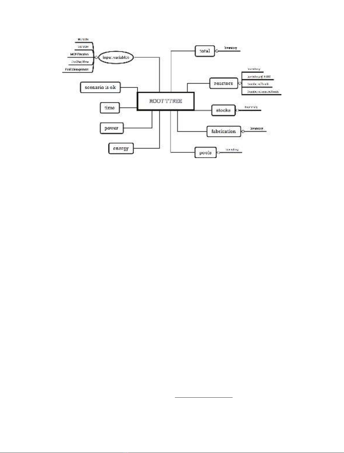
After N CLASS simulations, a single file containing
all the run informations is built. The output file is
handled by the analysis software ROOT [21]. A ROOT
TTree is built according to the structure represented in
Figure 2.
Scalar data are connected to oval shape since data
connected to square boxes are vectors in which index
represents the time step. For reactors output data, in
addition to inventory, the number of fresh fuel loading and
missed loadings is stored. In the defined design of
experiment, there is an empty cycle if there is not enough
plutonium to operate the PWR-MOx. The number of
missed loadings is then important for identifying runs with
lack of plutonium in the stockpile.
According to the accepted memory size dedicated to the
data file, around 10 000 simulations may be run. The set of
output files generated by CLASS simulations is around
300 GB and the final output file size is close to 15 GB. A
limitation coming from data storage memory may appear.
Indeed, a full analysis study may require many simulation
sets. To give an example, one could calculate the influence
of a model parameter on results provided by an output file.
This means to calculate and to store several high size files or
directories, just for one simple nuclear fleet. Among
solutions for the future of this methodology, we could
investigate on selecting data to store, define the appropriate
number of runs according to input variables and output
variability, etc.
Two independent input variable samples have been
generated from latin hypercube sampling (LHS) [22]. For
calculating Sobol’indices (see Sect. 4.2), a specific design of
experiment composed by 15 000 runs obtained from two
independent LHS samples of 1500 sets of input data has
been used. For output direct analysis (see Sects. 5 and 6)as
for preliminary analysis (see Sects. 4.3 and 4.4), 10 000
input data set have been sampled on a LHS.
3 The fuel cycle simulator CLASS
The fuel cycle model used in this work is the CLASS code
[23] which is a dynamic fuel cycle simulation tool developed
by CNRS
3
/IN2P3
4
in collaboration with IRSN
5
. The aim of
CLASS is to model an evolving electro-nuclear fleet. The
main output is the evolution of isotopes everywhere in the
fleet. An economic module [24] is also currently developed
to calculate the levelized cost of electricity of a nuclear fleet,
from the start until the dismantling.
3.1 CLASS principle
The CLASS model is a collection of C++ classes that
describes facilities in a nuclear fleet. The CLASS model has
been built around the reactor class that drives radioactive
material flows from reactor front to back end. Figure 3 lists
current existing facilities and links between them.
Five facilities, listed in Table 2 with associated user
defined parameters, are currently taken into account in
CLASS. From its starting time and at each new loading,
reactor requests a fresh fuel to the fabrication plant. The fuel
is irradiated inthe reactor and sent to the pool untilthe end of
the cooling time. The pool could beconnected toa separation
plant, that send separated elements to stocks. The end of the
path for any materials is a stock, that could be waste or not.
Fig. 2. Input and output data tree structure.
3
Centre National de la Recherche Scientifique.
4
Institut National de Physique Nucléaire et de Physique des
Particules.
5
Institut de Radioprotection et de Sûreté Nucléaire.
N. Thiollière et al.: EPJ Nuclear Sci. Technol. 4, 13 (2018) 5


![Câu hỏi ôn tập Truyền động điện [mới nhất]](https://cdn.tailieu.vn/images/document/thumbnail/2025/20250613/laphong0906/135x160/88301768293691.jpg)
![Giáo trình Kết cấu Động cơ đốt trong – Đoàn Duy Đồng (chủ biên) [Phần B]](https://cdn.tailieu.vn/images/document/thumbnail/2025/20251120/oursky02/135x160/71451768238417.jpg)


![Tài liệu học tập Công nghệ sản xuất và lắp ráp ô tô [mới nhất]](https://cdn.tailieu.vn/images/document/thumbnail/2025/20251231/kimphuong1001/135x160/50151767942304.jpg)

![Đề cương ôn tập môn Nguyên lý động cơ đốt trong [mới nhất]](https://cdn.tailieu.vn/images/document/thumbnail/2025/20251231/cuchoami2510/135x160/99621767694770.jpg)


