
Recurrent Neural Networks for Prediction
Authored by Danilo P. Mandic, Jonathon A. Chambers
Copyright c
2001 John Wiley & Sons Ltd
ISBNs: 0-471-49517-4 (Hardback); 0-470-84535-X (Electronic)
3
Network Architectures for
Prediction
3.1 Perspective
The architecture, or structure, of a predictor underpins its capacity to represent the
dynamic properties of a statistically nonstationary discrete time input signal and
hence its ability to predict or forecast some future value. This chapter therefore pro-
vides an overview of available structures for the prediction of discrete time signals.
3.2 Introduction
The basic building blocks of all discrete time predictors are adders, delayers, multipli-
ers and for the nonlinear case zero-memory nonlinearities. The manner in which these
elements are interconnected describes the architecture of a predictor. The foundations
of linear predictors for statistically stationary signals are found in the work of Yule
(1927), Kolmogorov (1941) and Wiener (1949). The later studies of Box and Jenkins
(1970) and Makhoul (1975) were built upon these fundamentals. Such linear structures
are very well established in digital signal processing and are classified either as finite
impulse response (FIR) or infinite impulse response (IIR) digital filters (Oppenheim
et al. 1999). FIR filters are generally realised without feedback, whereas IIR filters1
utilise feedback to limit the number of parameters necessary for their realisation. The
presence of feedback implies that the consideration of stability underpins the design of
IIR filters. In statistical signal modelling, FIR filters are better known as moving aver-
age (MA) structures and IIR filters are named autoregressive (AR) or autoregressive
moving average (ARMA) structures. The most straightforward version of nonlinear
filter structures can easily be formulated by including a nonlinear operation in the
output stage of an FIR or an IIR filter. These represent simple examples of nonlinear
autoregressive (NAR), nonlinear moving average (NMA) or nonlinear autoregressive
moving average (NARMA) structures (Nerrand et al. 1993). Such filters have immedi-
ate application in the prediction of discrete time random signals that arise from some
1FIR filters can be represented by IIR filters, however, in practice it is not possible to represent
an arbitrary IIR filter with an FIR filter of finite length.

32 OVERVIEW
nonlinear physical system, as for certain speech utterances. These filters, moreover,
are strongly linked to single neuron neural networks.
The neuron, or node, is the basic processing element within a neural network. The
structure of a neuron is composed of multipliers, termed synaptic weights, or simply
weights, which scale the inputs, a linear combiner to form the activation potential, and
a certain zero-memory nonlinearity to model the activation function. Different neural
network architectures are formulated by the combination of multiple neurons with
various interconnections, hence the term connectionist modelling (Rumelhart et al.
1986). Feedforward neural networks, as for FIR/MA/NMA filters, have no feedback
within their structure. Recurrent neural networks, on the other hand, similarly to
IIR/AR/NAR/NARMA filters, exploit feedback and hence have much more potential
structural richness. Such feedback can either be local to the neurons or global to the
network (Haykin 1999b; Tsoi and Back 1997). When the inputs to a neural network are
delayed versions of a discrete time random input signal the correspondence between
the architectures of nonlinear filters and neural networks is evident.
From a biological perspective (Marmarelis 1989), the prototypical neuron is com-
posed of a cell body (soma), a tree-like element of fibres (dendrites) and a long fibre
(axon) with sparse branches (collaterals). The axon is attached to the soma at the
axon hillock, and, together with its collaterals, ends at synaptic terminals (boutons),
which are employed to pass information onto their neurons through synaptic junc-
tions. The soma contains the nucleus and is attached to the trunk of the dendritic
tree from which it receives incoming information. The dendrites are conductors of
input information to the soma, i.e. input ports, and usually exhibit a high degree of
arborisation.
The possible architectures for nonlinear filters or neural networks are manifold.
The state-space representation from system theory is established for linear systems
(Kailath 1980; Kailath et al. 2000) and provides a mechanism for the representation
of structural variants. An insightful canonical form for neural networks is provided
by Nerrand et al. (1993), by the exploitation of state-space representation which
facilitates a unified treatment of the architectures of neural networks.2
3.3 Overview
The chapter begins with an explanation of the concept of prediction of a statistically
stationary discrete time random signal. The building blocks for the realisation of linear
and nonlinear predictors are then discussed. These same building blocks are also shown
to be the basic elements necessary for the realisation of a neuron. Emphasis is placed
upon the particular zero-memory nonlinearities used in the output of nonlinear filters
and activation functions of neurons.
An aim of this chapter is to highlight the correspondence between the structures
in nonlinear filtering and neural networks, so as to remove the apparent boundaries
between the work of practitioners in control, signal processing and neural engineering.
Conventional linear filter models for discrete time random signals are introduced and,
2ARMA models also have a canonical (up to an invariant) representation.
NETWORK ARCHITECTURES FOR PREDICTION 33
Σ
i
Discrete
Time
k
i=1
p
a y(k-i)
y(k)
^
(k-1)
(k-2)
y(k-2)
y(k-1)
y(k-p)
(k-p)
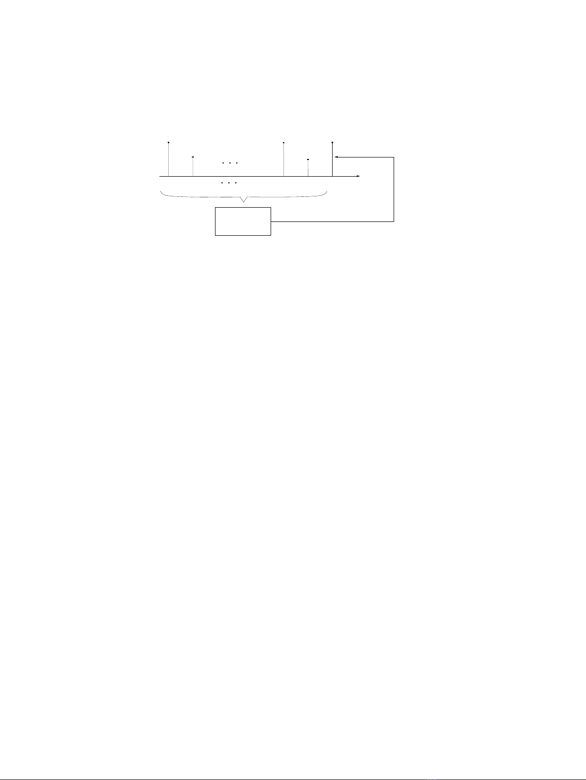
Figure 3.1 Basic concept of linear prediction
with the aid of statistical modelling, motivate the structures for linear predictors;
their nonlinear counterparts are then developed.
A feedforward neural network is next introduced in which the nonlinear elements
are distributed throughout the structure. To employ such a network as a predictor, it
is shown that short-term memory is necessary, either at the input or integrated within
the network. Recurrent networks follow naturally from feedforward neural networks
by connecting the output of the network to its input. The implications of local and
global feedback in neural networks are also discussed.
The role of state-space representation in architectures for neural networks is de-
scribed and this leads to a canonical representation. The chapter concludes with some
comments.
3.4 Prediction
A real discrete time random signal {y(k)}, where kis the discrete time index and
{·}denotes the set of values, is most commonly obtained by sampling some analogue
measurement. The voice of an individual, for example, is translated from pressure
variation in air into a continuous time electrical signal by means of a microphone and
then converted into a digital representation by an analogue-to-digital converter. Such
discrete time random signals have statistics that are time-varying, but on a short-term
basis, the statistics may be assumed to be time invariant.
The principle of the prediction of a discrete time signal is represented in Figure 3.1
and forms the basis of linear predictive coding (LPC) which underlies many com-
pression techniques. The value of signal y(k) is predicted on the basis of a sum of
ppast values, i.e. y(k−1),y(k−2),...,y(k−p), weighted, by the coefficients ai,
i=1,2,...,p, to form a prediction, ˆy(k). The prediction error, e(k), thus becomes
e(k)=y(k)−ˆy(k)=y(k)−
p
i=1
aiy(k−i).(3.1)
The estimation of the parameters aiis based upon minimising some function of the
error, the most convenient form being the mean square error, E[e2(k)], where E[·]
denotes the statistical expectation operator, and {y(k)}is assumed to be statistically

34 PREDICTION
wide sense stationary,3with zero mean (Papoulis 1984). A fundamental advantage of
the mean square error criterion is the so-called orthogonality condition, which implies
that
E[e(k)y(k−j)]=0,j=1,2,...,p, (3.2)
is satisfied only when ai,i=1,2,...,p, take on their optimal values. As a consequence
of (3.2) and the linear structure of the predictor, the optimal weight parameters may
be found from a set of linear equations, named the Yule–Walker equations (Box and
Jenkins 1970),
ryy(0) ryy(1) ··· ryy(p−1)
ryy(1) ryy(0) ··· ryy(p−2)
.
.
..
.
.....
.
.
ryy(p−1) ryy(p−2) ··· ryy(0)
a1
a2
.
.
.
ap
=
ryy(1)
ryy(2)
.
.
.
ryy(p)
,(3.3)
where ryy(τ)=E[y(k)y(k+τ)] is the value of the autocorrelation function of {y(k)}
at lag τ. These equations may be equivalently written in matrix form as
Ryya=ryy,(3.4)
where Ryy ∈Rp×pis the autocorrelation matrix and a,ryy ∈Rpare, respectively,
the parameter vector of the predictor and the crosscorrelation vector. The Toeplitz
symmetric structure of Ryy is exploited in the Levinson–Durbin algorithm (Hayes
1997) to solve for the optimal parameters in O(p2) operations. The quality of the
prediction is judged by the minimum mean square error (MMSE), which is calculated
from E[e2(k)] when the weight parameters of the predictor take on their optimal
values. The MMSE is calculated from ryy(0) −p
i=1 airyy(i).
Real measurements can only be assumed to be locally wide sense stationary and
therefore, in practice, the autocorrelation function values must be estimated from
some finite length measurement in order to employ (3.3). A commonly used, but
statistically biased and low variance (Kay 1993), autocorrelation estimator for appli-
cation to a finite length Nmeasurement, {y(0),y(1),...,y(N−1)}, is given by
ˆryy(τ)= 1
N
N−τ−1
k=0
y(k)y(k+τ),τ=0,1,2,...,p. (3.5)
These estimates would then replace the exact values in (3.3) from which the weight
parameters of the predictor are calculated. This procedure, however, needs to be
repeated for each new length Nmeasurement, and underlies the operation of a block-
based predictor.
A second approach to the estimation of the weight parameters a(k) of a predictor is
the sequential, adaptive or learning approach. The estimates of the weight parameters
are refined at each sample number, k, on the basis of the new sample y(k) and the
prediction error e(k). This yields an update equation of the form
ˆ
a(k+1)= ˆ
a(k)+ηf(e(k),y(k)),k0,(3.6)
3Wide sense stationarity implies that the mean is constant, the autocorrelation function is only
a function of the time lag and the variance is finite.
NETWORK ARCHITECTURES FOR PREDICTION 35
Z
−1
y(k) y(k−1)
(a)
b
a+ba
(b)
b
aab
(c)
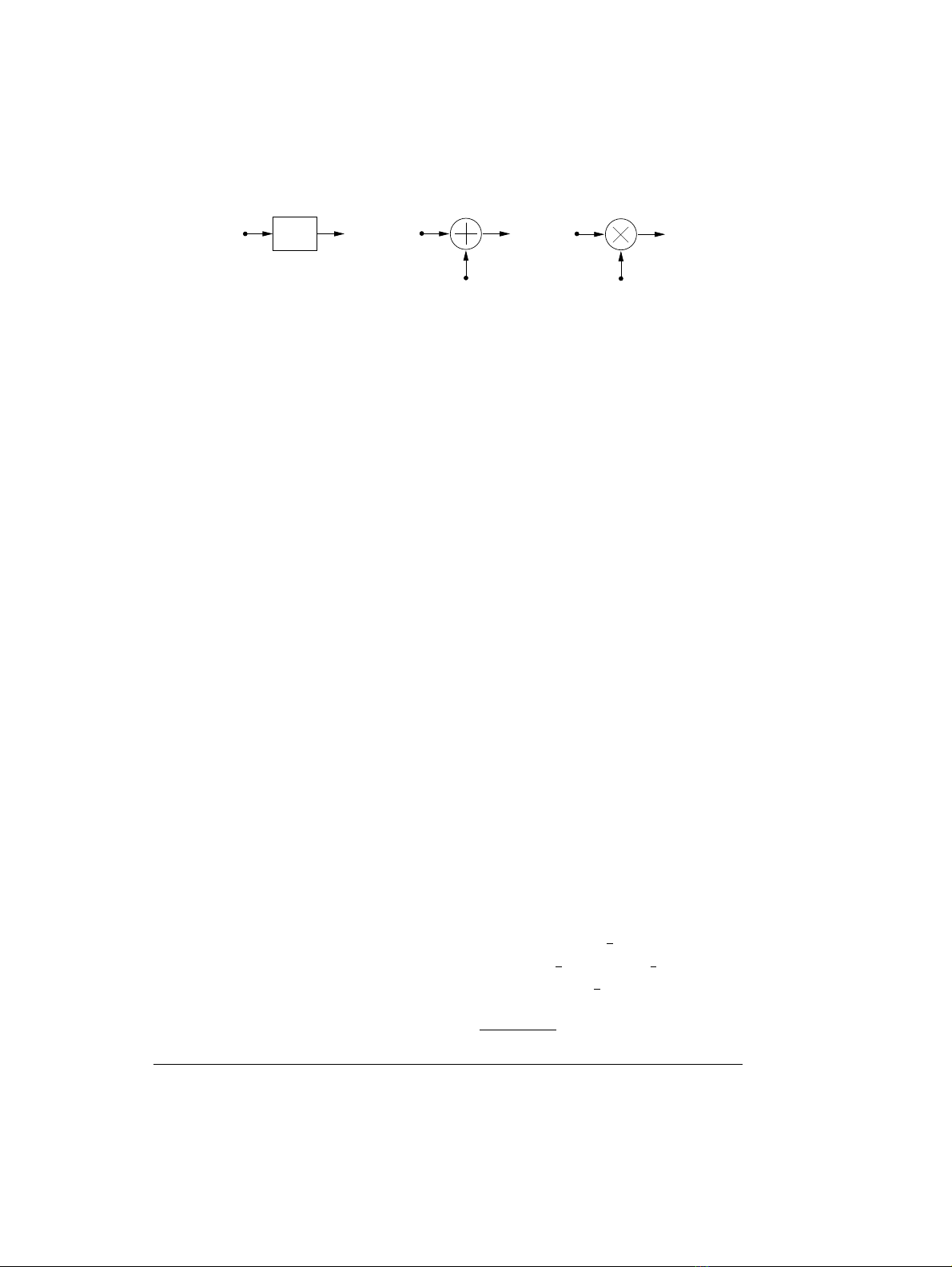
Figure 3.2 Building blocks of predictors: (a) delayer, (b) adder, (c) multiplier
where ηis termed the adaptation gain, f(·) is some function dependent upon the
particular learning algorithm, whereas ˆ
a(k) and y(k) are, respectively, the estimated
weight vector and the predictor input vector. Without additional prior knowledge,
zero or random values are chosen for the initial values of the weight parameters in
(3.6), i.e. ˆai(0)=0,orni,i=1,2,...,p, where niis a random variable drawn from a
suitable distribution. The sequential approach to the estimation of the weight param-
eters is particularly suitable for operation of predictors in statistically nonstationary
environments. Both the block and sequential approach to the estimation of the weight
parameters of predictors can be applied to linear and nonlinear structure predictors.
3.5 Building Blocks
In Figure 3.2 the basic building blocks of discrete time predictors are shown. A simple
delayer has input y(k) and output y(k−1), note that the sampling period is normalised
to unity. From linear discrete time system theory, the delay operation can also be
conveniently represented in Z-domain notation as the z−1operator4(Oppenheim et
al. 1999). An adder, or sumer, simply produces an output which is the sum of all the
components at its input. A multiplier, or scaler, used in a predictor generally has two
inputs and yields an output which is the product of the two inputs. The manner in
which delayers, adders and multipliers are interconnected determines the architecture
of linear predictors. These architectures, or structures, are shown in block diagram
form in the ensuing sections.
To realise nonlinear filters and neural networks, zero-memory nonlinearities are
required. Three zero-memory nonlinearities, as given in Haykin (1999b), with inputs
v(k) and outputs Φ(k) are described by the following operations:
Threshold: Φ(v(k)) = 0,v(k)<0,
1,v(k)0,(3.7)
Piecewise-linear: Φ(v(k)) =
0,v(k)−1
2,
v(k),−1
2<v(k)<+1
2,
1,v(k)1
2,
(3.8)
Logistic: Φ(v(k)) = 1
1+e
−βv(k),β0.(3.9)
4The z−1operator is a delay operator such that Z(y(k−1)) = z−1Z(y(k)).


%20--%3e%3cdefs%3e%3cstyle%3e%20.st0%20{%20fill:%20%23fff;%20}%20.st1%20{%20fill:%20%237800fa;%20}%20%3c/style%3e%3c/defs%3e%3cpath%20class='st1'%20d='M117.78,12.18H43.11c2.9,3.47,4.65,7.94,4.65,12.82,0,5.6-2.3,10.66-6.01,14.29h76.02l7.22-13.56-7.22-13.56Z'/%3e%3cg%3e%3cpath%20class='st0'%20d='M53.58,26.17h-.59v-1.46h.59v-4.96h2.83c1.78,0,2.67.94,2.67,2.82v5.76c0,1.87-.89,2.81-2.67,2.81h-2.83v-4.96ZM55.36,21.37v3.34h1.1v1.46h-1.1v3.34h1.01c.61,0,.91-.37.91-1.1v-5.93c0-.74-.3-1.1-.91-1.1h-1.01Z'/%3e%3cpath%20class='st0'%20d='M65.99,31.14h-1.8l-.31-2.07h-2.19l-.31,2.07h-1.64l1.82-11.39h2.62l1.82,11.39ZM65.28,18.04c-.25.46-.51.77-.75.94-.21.15-.47.22-.79.22-.26,0-.57-.07-.92-.22l-.38-.15c-.14-.05-.26-.07-.37-.07-.3,0-.53.18-.71.54l-.91-.68c.25-.46.51-.77.75-.94.21-.14.48-.21.79-.21.26,0,.57.07.92.21l.38.15c.14.05.26.07.37.07.3,0,.53-.18.71-.54l.91.68ZM61.91,27.52h1.73l-.87-5.76-.87,5.76Z'/%3e%3cpath%20class='st0'%20d='M74.53,26.89v1.52c0,1.91-.89,2.86-2.67,2.86s-2.67-.95-2.67-2.86v-5.93c0-1.91.89-2.86,2.67-2.86s2.67.95,2.67,2.86v1.11h-1.69v-1.22c0-.75-.31-1.12-.93-1.12s-.93.37-.93,1.12v6.15c0,.74.31,1.11.93,1.11s.93-.37.93-1.11v-1.63h1.69Z'/%3e%3cpath%20class='st0'%20d='M81.4,31.14h-1.8l-.31-2.07h-2.19l-.31,2.07h-1.64l1.82-11.39h2.62l1.82,11.39ZM75.9,19.2l1.52-1.91h1.71l1.51,1.91h-1.61l-.76-.95-.75.95h-1.61ZM77.32,27.52h1.73l-.87-5.76-.87,5.76ZM83.1,15.99l-1.76,1.91h-1.26l1.17-1.91h1.86Z'/%3e%3cpath%20class='st0'%20d='M84.86,19.75c1.78,0,2.67.94,2.67,2.82v1.48c0,1.87-.89,2.81-2.67,2.81h-.85v4.28h-1.79v-11.39h2.64ZM84.01,21.37v3.86h.85c.58,0,.87-.36.87-1.08v-1.71c0-.71-.29-1.07-.87-1.07h-.85Z'/%3e%3cpath%20class='st0'%20d='M93.51,19.75c1.78,0,2.67.94,2.67,2.82v1.48c0,1.87-.89,2.81-2.67,2.81h-.85v4.28h-1.79v-11.39h2.64ZM92.66,21.37v3.86h.85c.58,0,.87-.36.87-1.08v-1.71c0-.71-.29-1.07-.87-1.07h-.85Z'/%3e%3cpath%20class='st0'%20d='M98.8,31.14h-1.79v-11.39h1.79v4.88h2.03v-4.88h1.83v11.39h-1.83v-4.88h-2.03v4.88Z'/%3e%3cpath%20class='st0'%20d='M105.36,24.55h2.46v1.62h-2.46v3.34h3.09v1.63h-4.88v-11.39h4.88v1.63h-3.09v3.18ZM108.17,17.29l-1.76,1.91h-1.26l1.17-1.91h1.86Z'/%3e%3cpath%20class='st0'%20d='M112.2,19.75c1.78,0,2.67.94,2.67,2.82v1.48c0,1.87-.89,2.81-2.67,2.81h-.85v4.28h-1.79v-11.39h2.64ZM111.35,21.37v3.86h.85c.58,0,.87-.36.87-1.08v-1.71c0-.71-.29-1.07-.87-1.07h-.85Z'/%3e%3c/g%3e%3ccircle%20class='st1'%20cx='25'%20cy='25'%20r='20'/%3e%3cpath%20class='st0'%20d='M32.78,19.27c2.92,0,4.43,2.55,5.28,5.33l.71,2.17c.14.38-.33.75-.71.75h-5.61c.19-.33.24-.71.09-1.08l-.75-2.45c-.43-1.32-.99-2.64-1.79-3.77.75-.57,1.65-.94,2.78-.94h0ZM25,18.38c3.25,0,4.9,2.78,5.89,5.89l.76,2.45c.14.42-.33.8-.8.8h-11.69c-.42,0-.94-.38-.8-.8l.75-2.45c.99-3.11,2.64-5.89,5.89-5.89h0ZM25,11.35c1.74,0,3.11,1.37,3.11,3.11s-1.37,3.11-3.11,3.11-3.11-1.41-3.11-3.11,1.41-3.11,3.11-3.11h0ZM17.27,19.27c1.08,0,1.98.38,2.73.94-.8,1.13-1.37,2.45-1.74,3.77l-.8,2.45c-.14.38-.05.75.09,1.08h-5.56c-.42,0-.9-.38-.75-.75l.71-2.17c.9-2.78,2.41-5.33,5.33-5.33h0ZM17.27,12.91c1.51,0,2.78,1.27,2.78,2.83s-1.27,2.83-2.78,2.83-2.83-1.27-2.83-2.83,1.27-2.83,2.83-2.83h0ZM32.78,12.91c1.56,0,2.78,1.27,2.78,2.83s-1.23,2.83-2.78,2.83-2.83-1.27-2.83-2.83,1.27-2.83,2.83-2.83h0ZM27.07,28.56v.09c0,.57-.24,1.08-.61,1.46h0v.05c-.38.33-.9.57-1.46.57s-1.08-.24-1.46-.61h0c-.38-.38-.61-.9-.61-1.46v-.09h1.41v.09c0,.19.05.38.19.47v.05c.09.09.28.19.47.19s.38-.09.47-.19v-.05c.14-.09.24-.28.24-.47t-.05-.09h1.41ZM30.99,28.56v.09c0,1.65-.66,3.16-1.74,4.24-1.08,1.08-2.59,1.79-4.24,1.79s-3.16-.71-4.24-1.79l-.05-.05c-1.04-1.08-1.7-2.55-1.7-4.2v-.09h1.41v.09c0,1.27.47,2.4,1.27,3.25h.05c.85.85,1.98,1.37,3.25,1.37s2.4-.52,3.25-1.37c.85-.8,1.37-1.98,1.37-3.25v-.09h1.37ZM34.99,28.56v.09c0,2.78-1.13,5.28-2.92,7.07-1.79,1.79-4.29,2.92-7.07,2.92s-5.23-1.13-7.07-2.92c-1.79-1.79-2.92-4.29-2.92-7.07v-.09h1.41v.09c0,2.4.94,4.53,2.5,6.08,1.56,1.56,3.72,2.5,6.08,2.5s4.52-.94,6.08-2.5c1.56-1.56,2.5-3.68,2.5-6.08v-.09h1.41Z'/%3e%3c/svg%3e)