
http://www.iaeme.com/IJMET/index.asp 1962 editor@iaeme.com
International Journal of Mechanical Engineering and Technology (IJMET)
Volume 10, Issue 03, March 2019, pp. 1962–1973, Article ID: IJMET_10_03_198
Available online at http://www.iaeme.com/ijmet/issues.asp?JType=IJMET&VType=10&IType=3
ISSN Print: 0976-6340 and ISSN Online: 0976-6359
© IAEME Publication Scopus Indexed
AERODYNAMIC PROFILES FOR
APPLICATIONS IN HORIZONTAL AXIS
HYDROKINETIC TURBINES
J.D. Betancur G, J.G. Ardila M, A. Ruiz S
Department of Mechatronics and Electromechanical, Faculty of Engineering.
Instituto Tecnológico Metropolitano – ITM. Medellín, Antioquia, 050013, Colombia
E.L Chica A
Department of Mechanical Engineering, Faculty of Engineering.
Universidad de Antioquia- UdeA. Medellin, Antioquia, 050013, Colombia
ABSTRACT
Research in aerodynamics has allowed the creation of different profiles for certain
applications, reliably predicting the lift and drag coefficients by means of simulations
or experimental methods. In the field of wind and hydraulic power generation, they have
developed turbine rotors with improved performance and greater efficiency; several
researchers have evaluated the influence of the use of aero profiles on the operation of
hydrokinetic turbines through simulations and experimental tests. The main objective
of this review is to show the reader the importance of the proper choice of an aero
profile and its influence for the calculation during the design of rotor blades and the
performance of hydrokinetic turbines.
Key words: Design, Experimental, Hydraulic energy, Renewable energy, Simulation
Cite this Article: J.D. Betancur G, J.G. Ardila M, A. Ruiz S, E.L Chica A,
Aerodynamic Profiles for Applications in Horizontal Axis Hydrokinetic Turbines,
International Journal of Mechanical Engineering and Technology 10(3), 2019, pp.
1962–1973.
http://www.iaeme.com/IJMET/issues.asp?JType=IJMET&VType=10&IType=3
1. INTRODUCTION
The environmental and energy problems worldwide have forced researchers and professionals
to seek sustainable energy solutions. These have found in renewable sources, such as wind, sun
and water, viable alternatives to generate energy in a cleaner and more environmentally friendly
way. The energy extracted from water is the cheapest in the world; but, large hydroelectric
dams require large dams, this along with the civil works required have caused damage to the
environment and ecosystems, for this reason have been criticized [1]. That is why small
hydroelectric plants have become one of the most economical and environmentally friendly
sources of energy generation in rural areas [2]. Within the small hydroelectric plants, two ways
of harnessing the energy of water, hydrostatics and hydrokinetics stand out. The first is the way

J.D. Betancur G, J.G. Ardila M, A.Ruiz S, E.L Chica A
http://www.iaeme.com/IJMET/index.asp 1963 editor@iaeme.com
in which conventionally the energy has been generated by means of reservoirs that generate a
pressure head and then by means of a turbo machine the potential energy is extracted [3]. The
second form takes advantage of the kinetic energy of different water sources such as channels,
tides, oceans and rivers to turn turbo machineries and generate energy.
Hydrokinetic turbines are an emerging technology that has begun to gain strength and
recognition worldwide because they provide a low-cost energy solution and environmental
impact [4]. This technology is still in the development and research stage [5] and studies of
hydrodynamic characteristics are limited, for this reason more research is required on the
subject [6]. The optimal use of water is paramount for this type of turbines due to the low
density of electricity generation, for this reason there are studies that focus on improving the
efficiency and operation of hydrokinetic turbines using different aerodynamic profiles and
changes in curvature and the thickness [7]–[9]. In addition, the rotor blades are one of the most
important pieces for the conversion of energy in hydrokinetic turbines [10], for this reason the
design of the blade and the selection of the aero profile are essential for a maximum use of the
hydraulic resource [11].
In order to contribute to the development of this technology, this review focuses on showing
the importance of the selection of aerodynamic profiles, the ways in which they are studied,
due to the impact these profiles have on the performance of hydrokinetic turbines. In addition
to the selection of the profile, a review of the design, simulation and experimentation of the
hydrokinetic turbines of horizontal axis is carried out, providing the researchers of the subject
with a tool that allows them to have a criterion of choosing a profile and to know the different
techniques of design, simulation and experimentation of this type of turbines.
2. FORCES AND EFFECTS OF AERO PROFILES
There are different aero profiles suitable for certain speeds and applications [12], the difference
between one and the other is geometry. The majority of aerodynamic profiles are composed of
the parts. The leading edge or edge of entry is rounded and smooth and smooth; this shape
allows the profile to act efficiently at different inclination angles. Opposed to this is the trailing
edge or leakage, it is sharp and pointed, this in order to prevent the current from surrounding it,
except with an intense detachment of the boundary layer, to direct the current and allow a
reduction of the resistance to the advance. On the other hand, the rope is the line that goes from
the leading edge to the trailing edge. The line of curvature is equidistant between the extrados
and the intrados of the profile, the maximum distance from this to the rope defines the maximum
curvature of the profile (𝑐𝑚𝑎𝑥), which is usually between 25% and 50% of the rope. When the
curvature is less than 15% of the chord, the profile is said to be symmetrical and the thickness
distribution is the distance between the extrados and the intrados, normally this line of curvature
is a smooth curve between 20% and 40% of the chord [13].
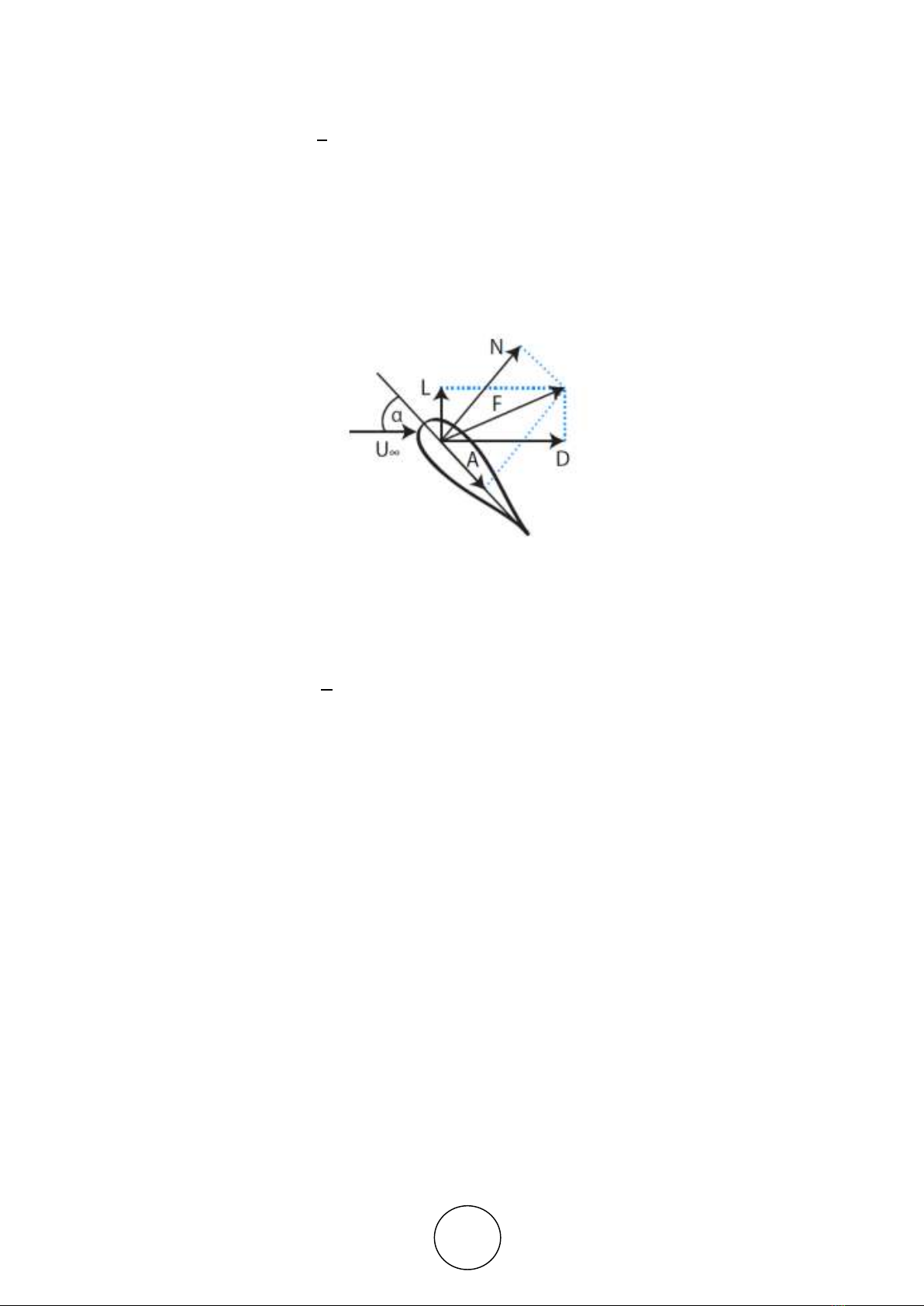
In an aero profile the flow travels the extrados at a higher speed producing a lower pressure
in this area; as in the intrados the distance is lower, lower speeds are produced, therefore, higher
pressures than in the upper part; this pressure difference generates the lift force (L). In the same
direction of flow, with speed 𝑈∞, a drag force (D) is generated. The coordinate vectors, A and
N, have as a reference plane the string of the aero profile, which can have an inclination (α)
with respect to the flow, called angle of attack. When combining the drag force and lift, a force
(F) is produced as seen in the Figure 1.
The sustentation (L) is the force that is generated on the aero profile when it crosses a fluid,
it is of direction perpendicular to the velocity of the flow; this force is responsible for keeping
airplanes in the air and turning the vast majority of wind and hydraulic turbines. The expression
(1) allows calculating the lift force.
Aerodynamic Profiles for Applications in Horizontal Axis Hydrokinetic Turbines
http://www.iaeme.com/IJMET/index.asp 1964 editor@iaeme.com
𝐿= 1
2𝜌𝑉2𝐴𝐶𝐿 (1)
Where:
L is the lift force [N].
ρ is the fluid density [kg m-3].
V is the velocity [m s-1].
A is the body reference area (also called "wing surface") [m2].
CL is the lift coefficient.
Figure 1. Aero profile forces.
The drag (D), also called fluid friction, occurs between the aero profile and the fluid through
which it moves, acts against the movement and is the sum of all the aerodynamic or
hydrodynamic forces in the direction of flow. Equation (2) allows calculating the drag force.
𝐃= 𝟏
𝟐𝛒𝐕𝟐𝐀𝐂𝐃 (𝟐)
Where:
D is the drag force [N].
CD is the drag coefficient.
Then the aerodynamic and hydrodynamic profiles are subjected to different loads, and as a
result are obtained forces associated with the production or consumption of mechanical energy;
Some forces such as lift and drag have been studied by [14]. Yavuz and others, developed a
study on two profiles NACA4412-NACA6411, in which they looked for the angle of attack
where the relation CL against CD was maximum, as well as points where the CL achieved its
highest values, finding that the optimal angles of attack were between 10° and 24° for both
profiles [15]. Then they made a comparison between the results obtained experimentally with
the turbine designed and those found numerically, obtaining an error lower than 7%. On the
other hand, Goundar used an S1210 hydro profile and showed that increasing the curvature by
20% resulted in a new hydro profile named HF-Sx, in which he showed a significant
improvement in the lift coefficient at different angles of attack studying it to a Reynolds
190.000.
Singh and Choi used the optimal conditions of two hydroprofiles, S914 and DU-91-W2-
250, to build a new one called MNU26, which had a thickness of 26% with respect to the chord
[16]. In another study, Kim, verified the behavior of the drag and lift coefficients for Reynolds
from 0,1 to 1.4 million, in profiles NACA63421 and MNU26 to find the optimal relationship
that would allow him to choose the best profile and the optimal angle of attack to a given regime
[17]. Like the previous ones, other authors have developed their own hydro profiles and have

J.D. Betancur G, J.G. Ardila M, A.Ruiz S, E.L Chica A
http://www.iaeme.com/IJMET/index.asp 1965 editor@iaeme.com
studied the lift and drag coefficients at different angles of attack, comparing their results with
commercial hydro profiles, obtaining the optimum L/D ratio with respect to some angle of
attack, for example, for Goundar and Ahmed they studied it with respect to a 9 ° angle [18].
Another study, carried out in Mexico, to evaluate the loads on a vane, obtaining the coefficients
of lift and drag, experimentally, in a wind tunnel [19]. Others have studied the lift coefficient
and the pressure coefficient for an S809 hydro profile, finding that for a Reynolds of one million
the best angle of attack was 8.2 °[20].
3. METHODOLOGIES FOR THE STUDY OF AERO PROFILES
3.1. Numerical Methodologies
The discretization of the volumes of control is key to the solution of problems by means of
finite element programs, when a good discretization is carried out the simulation results are
usually more precise and adjusted to the experimental ones. Below, some important aspects for
the discretization of the geometries are presented.
The mesh is a set of lines that divide an element or geometry creating cells or smaller areas;
they are connected with the adjacent elements to form finite element volumes. Meshing is one
of the most important steps in the simulation, since the phenomena of interest for the study can
be calculated accurately and efficiently through the mesh. For this reason, authors such as Lee,
Chung and Baek used hexahedral meshes [21].
Rainbird generated a mesh of 140,000 elements around a NACA0018 profile with an inflow
in quadrilaterals near the wall of the aero profile.This was done to capture, in detail, the velocity
and pressure gradients that are generated near this area [22], in the periphery of inflation larger
triangular elements were generated, this was done in order to decrease the number of elements
in areas that are not of interest to the study and thus save computation resources. Table 1
describes different numerical studies performed on profiles, presenting the profiles, their sizes
and the density of their meshes.
Table 1 Profiles used in different numerical studies and density of their meshes.
Author
Geometry
Chord size [mm]
Elements number
[Millions]
[23]
NREL S814
150
2.5
[24]
NACA0018/0021
1000
0.51
[25]
NACA0018
1000
0.139
[26]
NACA0012/ 0015/ 0020/ 0021
1000
0.446
The quality of the elements in a mesh is a factor that influences the precision of the simulation
results, for this reason there are several metrics that indicate the elements of a mesh quality, the
most important are the obliquity and the elements orthogonality. The obliquity says how similar
the mesh cells are to the ideal shape (equilateral prisms and hexahedrons). The quality ranges
for the obliquity are of acceptability when the maximum value is between 0.80 and 0.94. The
mesh elements must have a maximum acceptable obliquity to facilitate the solution
convergence. The second metric indicates the orthogonality between the sides of a face or the
faces of a cell, the ranges for orthogonal quality establish a minimum acceptable obliquity
between 0.15 and 0.20.
The Computational Fluid Dynamics (CFD) programs are used to perform fluid simulations
such as water and air, since it is an inexpensive way to obtain results that approximate the real
ones, for this reason several authors have used, in their investigations, programs CFD to solve

Aerodynamic Profiles for Applications in Horizontal Axis Hydrokinetic Turbines
http://www.iaeme.com/IJMET/index.asp 1966 editor@iaeme.com
physical phenomena [27] [28] [29] [30]. Turbulence models are mathematical expressions that
represent the physical phenomena of flows based on the Navier-Stokes equations. There are
three approaches to calculate the turbulence of a flow, the Direct Numerical Simulation (DNS),
Large Eddy Simulation (LES) and Reynolds Averaged Navier-Stokes Simulation (RANS) [31],
the first two are unworkable and impractical for the industry due to their high computational
cost, while the third is widely used for its low computational cost, effectiveness and accuracy.
Within the RANS models there are two large groups of turbulence models that are frequently
used for accuracy and computational cost, these are k-ε and k-ω, both models have two
additional transport equations to the Navier-Stokes model , one for the turbulent kinetic energy
(k) and the other for the energy dissipation rate (ε u ω).
The turbulence model k-ω SST has shown certain advantages over the k-ε since it solves in
a more precise way the phenomena that occur in the viscous sublayer (layer closest to the wall).
This attribute is very useful because it allows to capture phenomena such as the detachment of
the boundary layer, as well as the pressures and forces that are generated near the wall of the
aero profile [10] [32]. Table 2 shows some authors who have used the k-ω SST turbulence model
for their investigations.
The parameter y+ is a dimensionless number that relates other parameters of the fluid and the
flow with the distance that the first node of the mesh must have from the wall so that the
turbulence model captures the phenomena that occurred in the boundary layer. Commonly, for
the turbulence models, the y+ requirement is specified. The "y" value of the distance between
the wall and the centroid of the first mesh element can be calculated and defined according to
the expression (3). 𝐲= 𝐲+𝛍
√𝟏
𝟐(𝟎.𝟎𝟓𝟖𝐑𝐞−𝟎.𝟐)𝛒𝐔∞
𝟐
𝛒 𝛒 (𝟑)
The y+ depends on the turbulence model chosen as mentioned above, the density (ρ) and the
fluid viscosity (μ) are known, the Reynolds number (Re) is given by properties of the fluid and
the flow, and the length feature is the rope (L), as defined in (4).
𝐑𝐞=𝛒𝐕𝐋
𝛍 (𝟒)
The authors that used the family of the turbulence model k-ε used values to y+ (3) called less
than 300. On the other hand, those that used the family of the model k-ω reported values lower
than 1. Lee, Chung and Baek used a model of turbulence of this family called SST k-ω to correct
the lift coefficient of a S809 profile [21]. As Rainbird [22], in addition to maintaining the value
of y+ below 1 they used a growth rate of 1.1 for their study of aero profiles used in a wind
turbine. Table 2 reports the turbulence models and the y+ used by several researchers.
Table 2 Turbulence model k-ω and Y+ in different investigations.
Author
Geometry
Turbulence
model
Y+
Fluid


![Tài liệu học tập Hệ thống điều khiển điện - khí nén và thủy lực [mới nhất]](https://cdn.tailieu.vn/images/document/thumbnail/2021/20211005/conbongungoc09/135x160/811633401135.jpg)
![Tính chọn lắp ghép tiêu chuẩn giữa áo trục và trục chân vịt tàu thủy [chuẩn nhất]](https://cdn.tailieu.vn/images/document/thumbnail/2021/20210219/caygaocaolon10/135x160/5291613732560.jpg)

![Đề thi Kỹ thuật lập trình PLC: Tổng hợp [Năm]](https://cdn.tailieu.vn/images/document/thumbnail/2026/20260121/lionelmessi01/135x160/85491768986870.jpg)

![Đề thi cuối học kì 1 môn Máy và hệ thống điều khiển số năm 2025-2026 [Kèm đáp án chi tiết]](https://cdn.tailieu.vn/images/document/thumbnail/2025/20251117/dangnhuy09/135x160/4401768640586.jpg)


![Tự Động Hóa Thủy Khí: Nguyên Lý và Ứng Dụng [Chi Tiết]](https://cdn.tailieu.vn/images/document/thumbnail/2025/20250702/kexauxi10/135x160/27411767988161.jpg)


