
HPU2. Nat. Sci. Tech. Vol 03, issue 03 (2024), 27-34.
HPU2 Journal of Sciences:
Natural Sciences and Technology
Journal homepage: https://sj.hpu2.edu.vn
Article type: Research article
Received date: 23-7-2024 ; Revised date: 30-9-2024 ; Accepted date: 22-10-2024
This is licensed under the CC BY-NC 4.0
27
Algebraic method for image reconstruction in ultrasonic tomography
The-Lam Nguyen
*
, Quang-Huy Tran
Hanoi Pedagogical University 2, Vinh Phuc, Vietnam
Abstract
Ultrasound tomography is crucial due to its capability to deliver detailed, real-time, and non-invasive
imaging. This is essential for early diagnosis, treatment planning, and guiding medical procedures. Its
affordability, portability, and safety make it a versatile tool in medical and non-medical fields alike,
driving ongoing advancements in technology and applications. The Distorted Born Iterative Method
(DBIM) is an advanced technique used in ultrasound tomography to iteratively restore images,
improving upon the standard Born approximation by addressing some of its limitations. However, the
DBIM also has its own set of disadvantages when used for iterative image restoration, resulting in
computational complexity, noise sensitivity, convergence issues, etc. In this paper, we introduce a new
method for image reconstruction in ultrasound tomography by using the algebraic method. The
numerical results indicate that this method has a shorter computational time and achieves high-
resolution reconstructions and accurate solutions.
Keywords: Algebraic method, ultrasonic tomography, image reconstruction, incident pressure,
scattering pressure
1. Introduction
Ultrasound tomography (UT) [1] is a medical imaging technique that uses sound waves to create
three-dimensional (3D) images of internal organs, tissues, and blood flow. It's similar to the more
common CT scan (computed tomography) but uses sound waves instead of X-rays. Unlike traditional
ultrasound which provides 2D slices, UT builds a 3D image similar to a CT scan. It achieves this by
using sound waves instead of X-rays. During a UT exam, a probe emits high-frequency sound waves
that travel through the body. The interaction of these waves with tissues – reflection, refraction,
scattering and absorption – is measured by multiple detectors positioned around the target area.
Powerful computers then process this complex data to create a detailed 3D image. In the case of
*
Corresponding author, E-mail: nguyenthelam@hpu2.edu.vn
https://doi.org/10.56764/hpu2.jos.2024.3.3.27-34

HPU2. Nat. Sci. Tech. 2024, 3(3), 27-34
https://sj.hpu2.edu.vn 28
interaction with objects with size in order to wavelength, the ultrasound will be scattered. For detecting
small cancer at the beginning of the period, this technique only focuses on the scattering of ultrasound.
The advantages of UT are significant. Unlike X-rays, ultrasound is safe for repeated use, making it ideal
for monitoring conditions or following up on treatment. Additionally, UT offers superior contrast for
soft tissues, potentially improving the detection of tumors or abnormalities compared to traditional
ultrasound.
Based on the first-order Born approximation [2], ultrasonic tomography is one of these strategies
[3], which is known to be a potentially valuable method of imaging objects with a similar acoustical
impedance to that of the surrounding homogeneous medium such as in soft tissue characterization [4]
and underwater acoustics [5]. But difficulties arise when it is proposed to obtain quantitative tomograms
using acoustical parameters such as the velocity or the attenuation of the wave or tomograms of more
highly contrasted media such as in the case of hard tissues [6], industrial process tomography [7], [8],
etc. Finding solutions here involves either using iterative schemes [9] and/or performing extensive
studies on the limitation of the first-order Born approximation [10]. A high-order Born tomographic
method named distorted Born diffraction tomography is also studied in [11], [12].
The theoretical development of the first-order Born tomographic method is asymptotic, as
described using Green's function in the case of a homogeneous medium. The unknown object function,
which has been extended to the case of weakly contrasted and weakly heterogeneous media, is linearly
related to the measured field via a Fourier transform, and the inverse problem is related to the filtered
back-projections algorithm [13]. In the case of more highly contrasted media, this strategy was adapted
experimentally to take into account physical phenomena such as wave refraction, where the problem can
be reduced to the study of a fluid-like cavity buried in an elastic cylinder surrounded by water. Since
this iterative experimental method, which is known as compound ultrasonic tomography, gives excellent
results, the only limitations here are the heavy data processing required and the complex acoustical
signals resulting from the multiple physical effects involved.
Nonlinear inversion methods with higher-order levels of approximation have therefore been
investigated, including the distorted Born iterative method [14], [15], which is generally applied to
solving electromagnetic [16]–[18] and optical [19] inverse scattering problems. However, very few
ultrasonic experimental reconstructions are available in the literature [20]. The ultrasonic distorted Born
diffraction tomography approach based on this iterative method makes it possible to obtain quantitative
images.
However, UT is still under development. Challenges include complex calculations and the bending
of sound waves within the body. Advancements in computing power and new UT designs are paving the
way for wider clinical applications. While not yet a replacement for established techniques, UT holds
promise for a future where safe, detailed imaging of soft tissues is readily available. There are a couple
of methods used for reconstructing ultrasonic tomography images as filtered back projection, distorted
Born iterative method (DBIM), etc. where DBIM is one approach for reconstruction in UT. It can
handle objects with large variations in sound speed, which is important for biological tissues and
achieves high-resolution reconstructions compared to some simpler methods. Due to DBIM is being an
iterative method, it can be computationally expensive, especially for complex objects and, in some
cases, the iterative process might not converge to an accurate solution. Our algebraic methods are a
powerful tool for reconstructing these images from the collected data. Where the object is discretized
into a grid of pixels. Ultrasound waves travel through the object along specific paths. In each pixel, the
ultrasound may be scattered. The travel time or intensity of the waves is measured for each path. This
data is used to create a system of equations that relates the pixel values to the measured data. The
HPU2. Nat. Sci. Tech. 2024, 3(3), 27-34
https://sj.hpu2.edu.vn 29
algebraic methods then solve this system of equations to estimate the value of each pixel, building the
final image. This method can handle complex acquisition geometries where the sound source and
receiver may not follow a simple path. Solving large systems of equations can be computationally
expensive and gets singulars.
2. Algebraic Reconstruction Techniques
This method involves creating a mathematical model of the object and iteratively refining it based
on the acquired ultrasound data. This allows for more complex image reconstruction, especially when
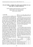
dealing with uneven material properties or curved surfaces. For collecting scattered data of UT in the
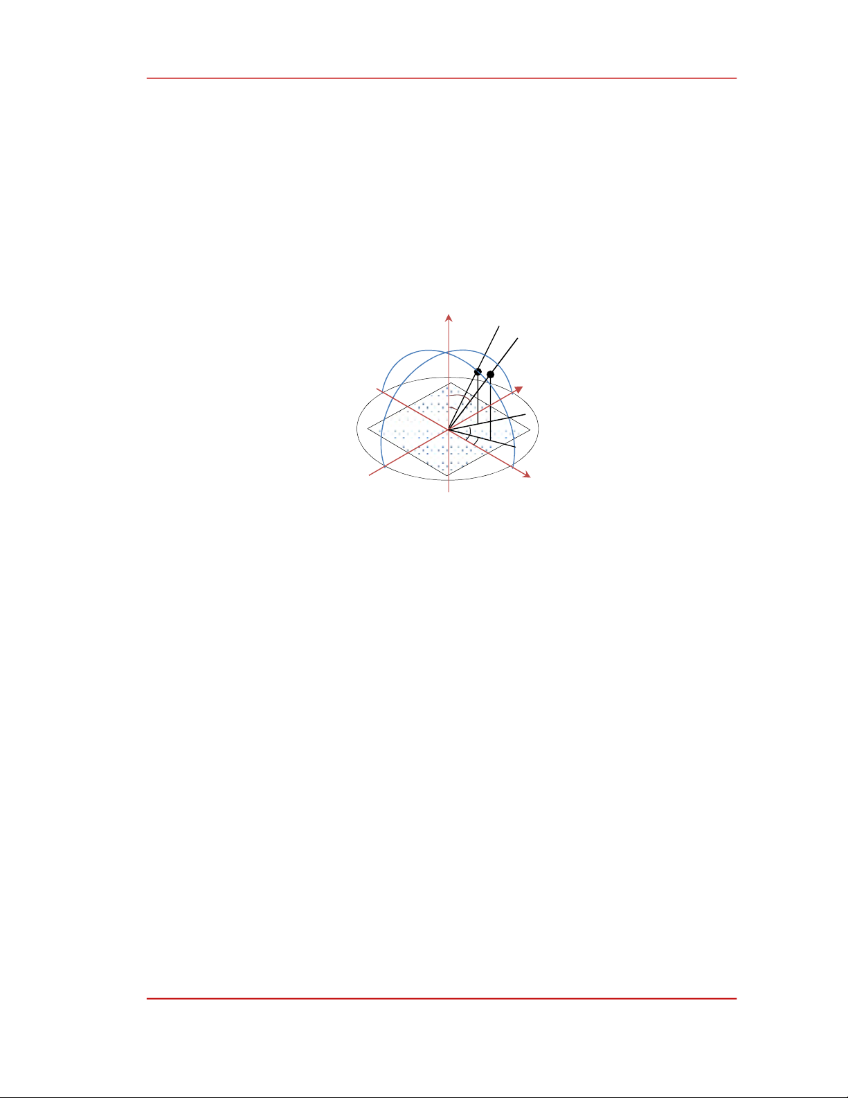
breast, we set up a configuration as Figure 1.
Figure 1. The configuration for ultrasonic computer tomography.
In this configuration, for convenience, we use a transducer and a receiver. They move on an upper-
haft sphere with a radius of R. The distance between them is constant when they move on the sphere
together. In the sphere coordinate system, the positions of the transducer are determined by the radius
R
, angles a
0
nd
0
. The positions of receivers are also determined by
1
,
R
and
1
.
The UT image is considered as a matrix of
N N
pixels. The element of the matrix is defined as
the scattering coefficient of soft tissue. These coefficients are equal to zero for objects with sizes that are
much greater than the wavelength of ultrasound. They are only different from zero for objects with size
in the order of the wavelength of ultrasound. For convenience, the object is defined simply as
0
0
0
0
0
1
for r r
O r for r r
a
a
(1)
where,
O r
is the matrix of UT,
r
is the position of a pixel,
0
r
is the position of an object on the
plane of the UST and a0 is the radius (size) of the object.
At the receiver, the pressure of the ultrasound is given
1
N N
inc scr
i i
i
p p O p
(2)
where,
inc
p
is the incident sound directly from the transducer,
i
O
is the scattering coefficient of the i-th
pixel and
scr
i
p
is the scattered sound by i-th pixel of the UT image. The incident sound
inc
p
is
estimated as
z
Receiver
0
Transducer
y
1
1
0
x
HPU2. Nat. Sci. Tech. 2024, 3(3), 27-34
https://sj.hpu2.edu.vn 30
.exp
inc
o
p d p d
(3)
where,
o
p
is the amplitude of sound,
is the attenuation coefficient and d is the distance from the
transducer to the receivers. The scattered sound
scr
i
p
is estimated
0 1
0.exp
scr
i i i
p p r r
(4)
where,
0
i
r
is the distance from the transducer to the i-th pixel and
1
i
r
is the distance from the i-th pixel
to the receivers. Let,
inc
b p p
, 1
scr
i
a p
and ,
i i
x O
. Rewriting (2) in the matrix form, we have
1
1
11 12 11
2 22 222
1 2
...
...
...
... ..
.
.
..
. ... .
...
. .
NN
NN
NN N
NN NN N
NN NN
a a a b
a a a b
b
x
x
a a a x
(5)
The elements of matrix b may be obtained from experiments (receivers) and elements of matrix a
are obtained from the configuration of UT. Dividing matrix b by matrix a, we may obtain matrix x. The
matrix of column x contains information on the UT image, therefore, it should be rearranged in the form
of a square matrix
11 12 1
21 22 2
1 2
...
...
... ... ... ...
...
N
N
N N NN
O
x x x
x x x
x x x
(6)
3. Computation
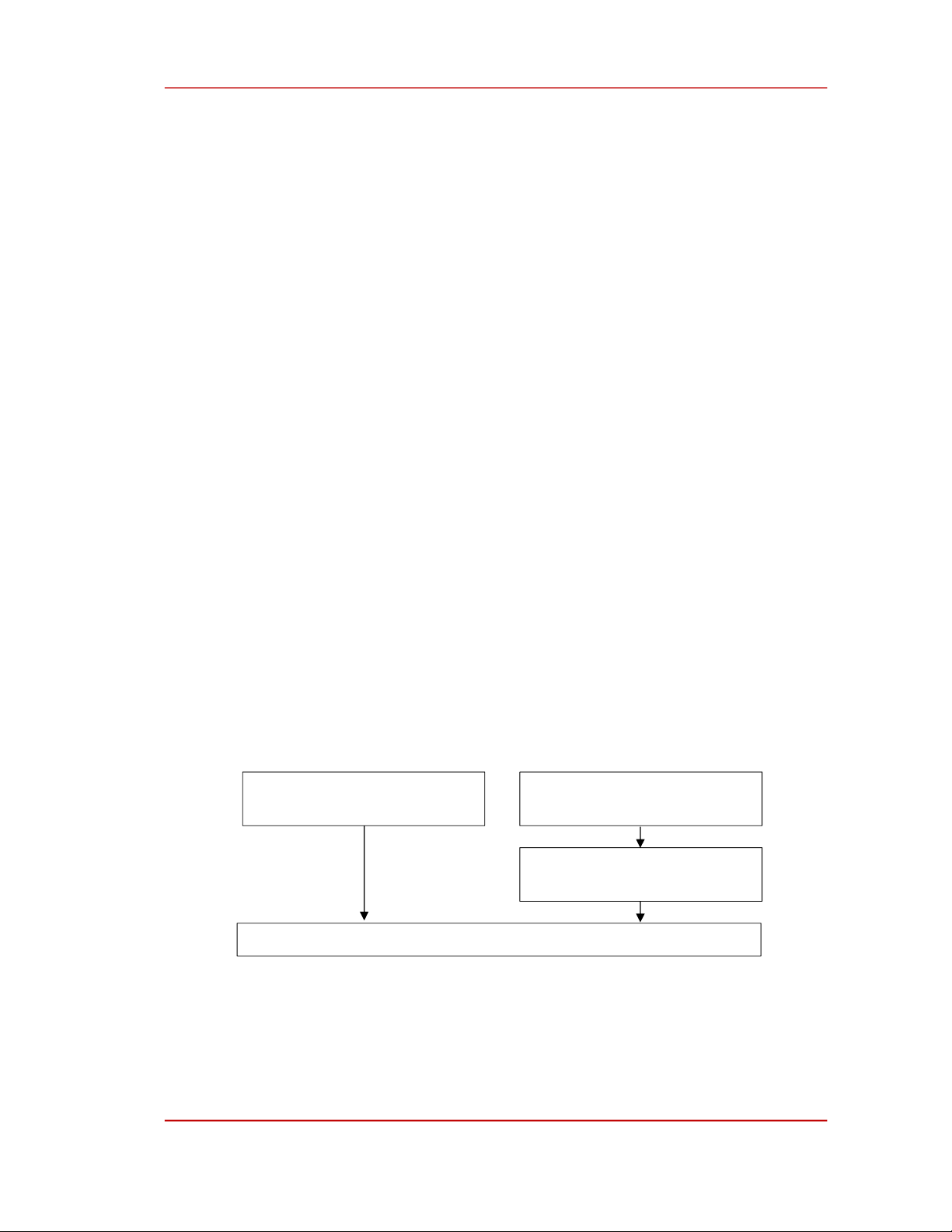
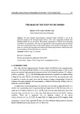
To demonstrate our model, two problems are set up and solved as Figure 2. The first is the
collection of data from receivers. In the experiment, data is the received pressure of scattering
ultrasound on the detectors. In the simulation, we assume that the data is received from (2) via a simple
algorithm.
Figure 2. The follow chart of computation.
The second problem is a reconstruction of UT. From (2), the total scattering pressure from pixels at
one position of the receiver is given
1
N N
n n n scr n
Total Data inc i i
i
P P P O P
(7)
Calculation of incident pressure
p_inc on the detectors
Calculation of scattering pressure
p_scr from each pixel
Calculation of total scattering
pressure
Data of detector
HPU2. Nat. Sci. Tech. 2024, 3(3), 27-34
https://sj.hpu2.edu.vn 31
where,
n
Data
P
is the received data at position n, and
n
inc
P
is the incident wave pressure directly from the
transducer. Since the distance between the transducer and the receiver is constant, therefore
n
inc
P const
can be calculated via equation (3). The
scr n
i
P is the scattering wave pressure from each
pixel i-th at the position of the receiver n, they can be calculated via configuration of measurements.
From (7), for 1
n N N
, we have a system of linear equation.
4. Simulation and discussion
The parameters of configuration are set up for detecting small cancers of the breast. The size of these
cancers is in the order of sound wavelength. They usually are in the early stage of cancer and cannot be
detected by typical ultrasonic images. The size of UT is
10 10
L L cm cm
and the radius of sphere
5
R cm
(size of breast); the matrix of UT is set up as
8 8
N N
and
13 13
N N
pixel
respectively. The breast may be considered as soft tissue; therefore, the attenuation coefficient of the
breast is chosen as
= 1 in the range from 0.75 (soft tissue) to 1.3 (muscle). The original amplitude of the
sound source 0
100%
p
. The displacements of the transducer and receiver are set up by
0 1
8
and 0 1
8
.
For i = 1 to N
For j = 1 to N
0
1 *2 /
i
i N
1 0
i i
0
1 * / 2
j
j N
1 0
i i
End.
End.
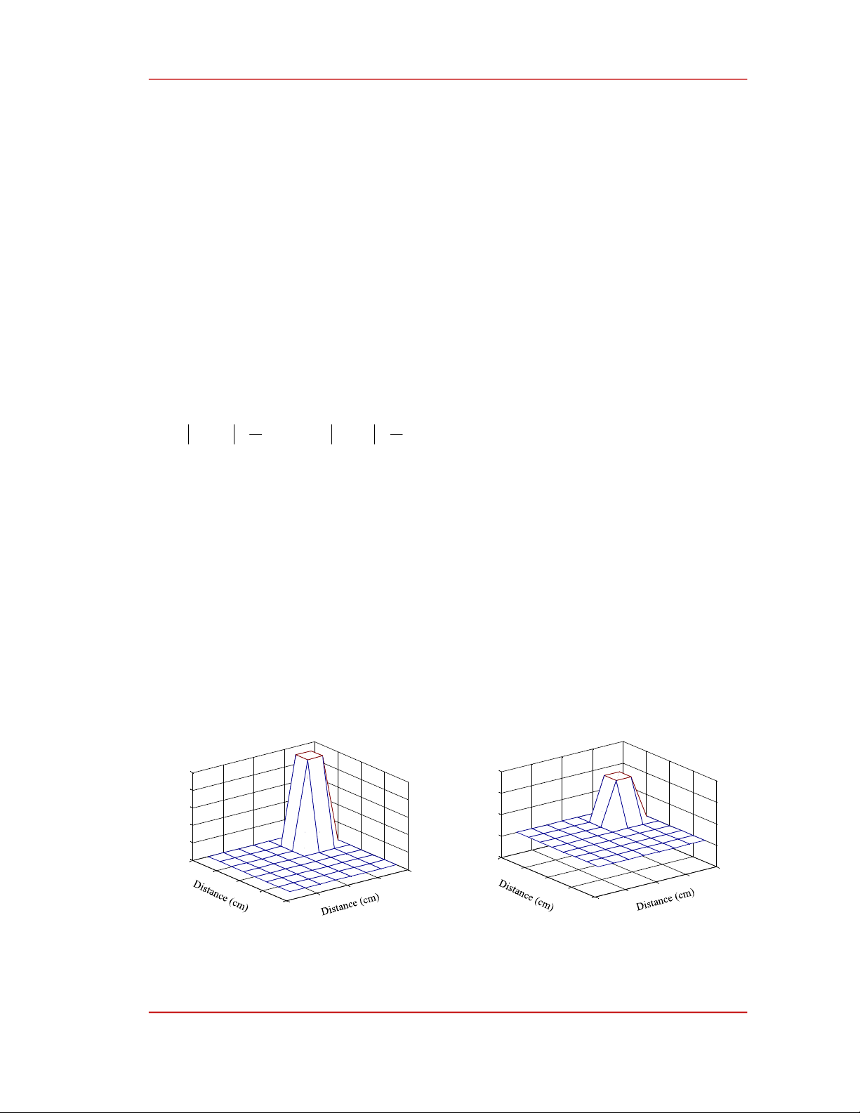
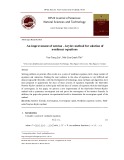
The matrix of the UT is reconstructed as Figure 4
8
N
and Figure 6
13
N, they are very fit
in comparison with the idea target matrixes with the same size in Figure 3
8
N
and Figure 5
13 .
N
Figure 3. The idea target matrix with
8
N
.
Figure 4. The reconstructed matrix by the algebraic
method with
8.
N
0
2
4
6
8
0
2
4
6
8
0
0.2
0.4
0.6
0.8
1
0
2
4
6
8
0
2
4
6
8
-0.5
0
0.5
1
1.5
Percent of sound
contrast
Percent of sound
contrast


![Bài giảng Vật lý đại cương Chương 4 Học viện Kỹ thuật mật mã [Chuẩn SEO]](https://cdn.tailieu.vn/images/document/thumbnail/2025/20250925/kimphuong1001/135x160/46461758790667.jpg)