
Hindawi Publishing Corporation
EURASIP Journal on Image and Video Processing
Volume 2008, Article ID 741290, 10 pages
doi:10.1155/2008/741290
Research Article
A Motion-Adaptive Deinterlacer via Hybrid Motion Detection
and Edge-Pattern Recognition
Gwo Giun Lee,1Ming-Jiun Wang,1Hsin-Te Li,2and He-Yuan Lin1
1Department of Electrical Engineering, National Cheng Kung University, 1 Ta-Hsueh Road, Tainan 701, Taiwan
2Sunplus Technology Company Ltd, 19 Chuangsin 1st Road, Hsinchu 300, Taiwan
Correspondence should be addressed to Ming-Jiun Wang, n2894155@ccmail.ncku.edu.tw
Received 31 March 2007; Revised 25 August 2007; Accepted 13 January 2008
Recommended by J. Konrad
A novel motion-adaptive deinterlacing algorithm with edge-pattern recognition and hybrid motion detection is introduced. The
great variety of video contents makes the processing of assorted motion, edges, textures, and the combination of them very difficult
with a single algorithm. The edge-pattern recognition algorithm introduced in this paper exhibits the flexibility in processing both
textures and edges which need to be separately accomplished by line average and edge-based line average before. Moreover, predict-
ing the neighboring pixels for pattern analysis and interpolation further enhances the adaptability of the edge-pattern recognition
unit when motion detection is incorporated. Our hybrid motion detection features accurate detection of fast and slow motion in
interlaced video and also the motion with edges. Using only three fields for detection also renders higher temporal correlation for
interpolation. The better performance of our deinterlacing algorithm with higher content-adaptability and less memory cost than
the state-of-the-art 4-field motion detection algorithms can be seen from the subjective and objective experimental results of the
CIF and PAL video sequences.
Copyright © 2008 Gwo Giun Lee et al. This is an open access article distributed under the Creative Commons Attribution License,
which permits unrestricted use, distribution, and reproduction in any medium, provided the original work is properly cited.
1. INTRODUCTION
Interlaced scanning, or interlacing, which performs vertical-
temporal subsampling of video sequences was used to lower
the costs of video system and reduce transmission bandwidth
by half while retaining visual quality in traditional TV. One
common characteristic of many television standards evolv-
ing over time, such as PAL, NTSC, and SECAM, is interlaced
scanning. With recent advancements of digital TV (DTV),
high-definition TV (HDTV), and multimedia personal com-
puters, deinterlacing has become an important technique
which converts interlaced TV sequences into frames for dis-
play on progressive devices such as LCD TVs, plasma dis-
play panels, and projective TVs. Intrinsic to this interoper-
ability of the two seemingly separate domains is the con-
version of interlaced TV formats to progressive displays via
deinterlacers. Hence, the increased demand for research in
video processing systems to produce progressively scanned
video with high-visual quality is inevitable [1].
The deinterlacing problem can be stated as
po(i,j,k)=⎧
⎨
⎩
pi(i,j,k), ( j+k)%2 =0,
p(i,j,k), otherwise, (1)
where pi,
p,andpodenote the input, interpolated, and out-
put pixels, respectively. i,j,andkrepresent horizontal, verti-
cal, and temporal pixel indices. % is modulo operation. The
vertical-temporal downsampling structure of interlacing is
also explained in (1), in which
pindicates the missing point
due to interlacing.
The challenge of deinterlacing is to interpolate the miss-
ing points
pwith limited information and also to maintain
clear visual quality as well. However, visual defects such as
edge flicker, line crawling, blur, and jaggedness due to the in-
herent nature of interlaced sequences frequently appear and
produce annoying artifacts to viewers if deinterlacing is not
done properly.
The key concept of deinterlacing is to interpolate the
missing point with spatio-temporal neighbors that have the
highest correlation. A wide variety of deinterlacing algo-
rithms, following this principle, has been proposed in the last
few decades. A comprehensive survey can be found in [2].
We introduce several frequently used techniques, which are
helpful in understanding this paper, in the following.
Since pi(i,j−1, k), pi(i,j+1,k), and pi(i,j,k−1) are
the nearest neighbors of
p(i,j,k), they potentially have the
highest correlation. Two simple interpolation strategies, line
2 EURASIP Journal on Image and Video Processing
average (LA) and field insertion (FI), were hence proposed.
LA, an intra-interpolation method, interpolates
p(i,j,k)
with (pi(i,j−1, k), pi(i,j+1,k))/2. On the other hand, FI, an
inter-interpolation method, repeats pi(i,j,k−1) as
p(i,j,k).
LA and FI methods are so simple that they cannot handle
generic video contents. LA blurs vertical details and causes
temporal flickering. FI introduces line crawl of moving ob-
jects.
Another intra-interpolation method, called edge-based
line average (ELA) [3], was proposed to preserve edge sharp-
ness and integrity and avoid jaggedness of edges. ELA in-
terpolates a pixel along the edge direction explored by com-
paring the gradients of various possible directions. Although
ELA is capable of restoring the edges of interlaced video, it
also introduces “pepper & salt” noises when edge directions
are misjudged. Moreover, the weakness in recovering com-
plex textures is one of its drawbacks. Some variations of ELA,
such as adaptive ELA [4], enhanced ELA (EELA) [5], and ex-
tended intelligent ELA algorithm [6] were proposed to fur-
ther improve its performance.
Motion-adaptive methods [7–9]wereproposedtoalle-
viate the impact of motion so that the correlation of the
reference pixels for interpolation is higher. Motion-adaptive
deinterlacing employs motion detection (MD), and switches
or fades between filtering strategies for motion and non-
motion cases by calculating the differences of luminance
between several consecutive fields. A good survey on mo-
tion detection of interlaced video can be found in [10].
Motion detection requires field memories to store previous
fields and possibly future fields. With more fields and thus
more information, the detection accuracy is usually higher
at the cost of more field memory in VLSI implementation.
In motion-adaptive deinterlacing, intra-interpolation is se-
lected for motion cases, while inter-interpolation is used
for stationary scenes. The visual quality of motion-adaptive
methods highly relies on the correctness of motion informa-
tion. Textures make correct motion detection, especially the
detection of fast motion, even more difficult, since the verti-
cal and temporal high frequencies are mixed up in interlaced
video. It was reported in [11] that texture analysis by wavelet
decomposition can enhance the precision of motion detec-
tion. Motion-compensated methods [12–15]involvemotion
estimation [16–18] for filtering along the motion trajecto-
ries. They perform very accurate interpolation at the cost of
much higher hardware expenditure.
Rich video contents provide viewers with high-visual
satisfaction but complicate the deinterlacing process, since
different visual signal processing strategies should be ap-
plied to the video signals with more information. The
motion-adaptive method with FI and LA switches between
a vertical all-pass filter and a temporal all-pass filter and
hence provides a content-adaptive algorithm. However, the
adaptability of motion detection and intra-interpolation did
not draw much attention before. The earlier motion detec-
tion algorithms focused on accurate same-parity detection
but neglected the detection of fast motion. Moreover, in-
creasing the number of fields to obtain higher accuracy also
accompanies higher cost of memory hardware. On the other
hand, ELA-styled interpolations emphasized the sharpness of
Input
fields Hybrid
motion
detection
Motion-map
refining unit Motion
detector
Edge-pattern
recognition
unit
Field
insertion
Pixel interpolator
Deinterlacing
output
Figure 1: Block diagram of the proposed deinterlacing algorithm.
edges but ignored the importance of textures. The robustness
of these algorithms toward different video contents can still
be enhanced.
In this paper, we present a hybrid motion-adaptive dein-
terlacing algorithm (HMDEPR), which consists of novel hy-
brid motion detection (HMD) and edge-pattern recognition
(EPR) with emphasis on content-adaptive processing. HMD
is capable of detecting versatile motion scenarios by using
only three fields. EPR targets the interpolation of edges and
textures, which can not be handled by using either LA or ELA
alone. The experimental results indicate that our HMD, EPR
for intra-interpolation, and our deinterlacing algorithm all
exhibit higher robustness toward assorted video scenes. This
paper is organized as follows. Section 2 presents our motion-
adaptive deinterlacing algorithm. The experimental results
and performance comparison are shown in Section 3.The
conclusion of this research is drawn in Section 4.
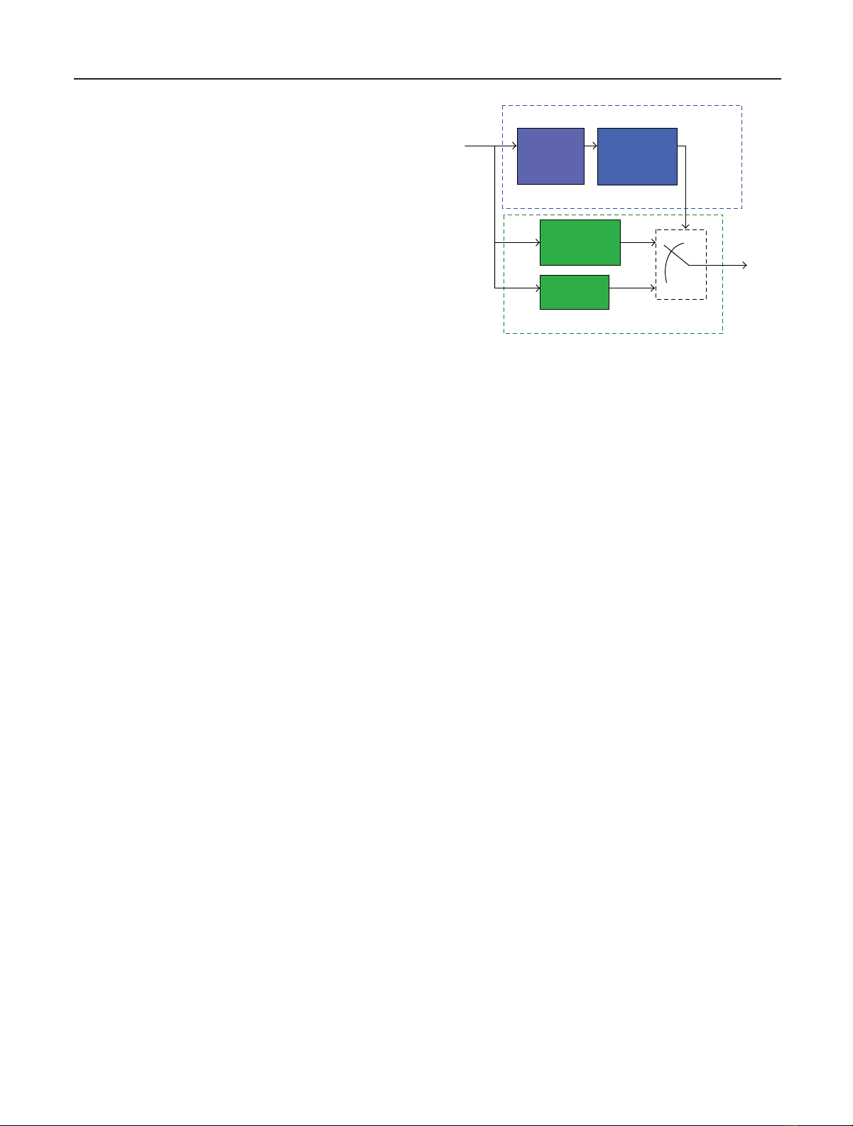
2. THE PROPOSED DEINTERLACING ALGORITHM
We introduce a deinterlacing algorithm which adapts to the
motion, texture, and edge contents of the video sequence.
The overall algorithm, shown in Figure 1, consists of a mo-
tion detector and a pixel interpolator. Our motion detector
employs HMD and a refinement unit. The interpolator in-
cludes EPR and FI. FI is used when a pixel is detected as sta-
tionary, and EPR is used otherwise. HMD and EPR are tac-
tically designed to achieve high adaptability towards a great
variety of motion, textures, and edges.
2.1. Motion detection
The goal of motion detection is to identify motion scenes
and enable intra-interpolation. We employ a hybrid motion
detector (HMD) which requires the pixel data of only three
fields. The pseudo-codes of the HMD are shown in Figure 2.
The three conditions are dedicated to the detection of slow
motion, fast motion, and motion with edges.
The first condition of HMD is traditional 3-field motion
detection. The 3-field motion detection is capable of detect-
ing most of the motion scenarios except the case in which
Gwo Giun Lee et al. 3
diff1=abs(a−b)
diff2=abs[b−(c+d)/2]
diff3=abs[b−(g+h)/2]
diff4=abs[a+(e+f)/2−b−(g+h)/2]
if diff1>TH1 ⊲1st condition
flag ←− motion
else if diff2>TH1 AND diff3<TH2 ⊲2nd condition
flag ←− motion
else if diff4>TH3 ⊲3rd condition
flag ←− motion
else
flag ←− stationary
(a)
g
c
e
b
d
a
hf
X
Scan line
Time
n−1nn+1
(b)
Figure 2:Theproposedhybridmotiondetectionalgorithm.(a)
Pseudocodes, (b) pixel definition.
moving objects or backgrounds only appear in field nbut
neither in field n−1norfieldn+1.Thisissupportedby
the fact that near-zero difference of a−bin this case falsely
indicates no motion. Hence, in the second condition, we fur-
ther take the line average result as a temporarily interpolated
point and detect motion between two consecutive fields un-
der the condition that the vertical variation diff3is small.
This 2-field motion detection operates on the previous field
rather than the next field so as to coherently work with FI
from the previous field in stationary scenes. The proposed
HMD combines the merits of 3-field motion detection and
2-field motion detection, which are good detection accuracy
for stationary pixels, and the ability to detect the very fast
motion that cannot be detected by 3-field motion detection,
respectively. The third condition enhances the detection ac-
curacy of edges. The reason will be explained in Section 3.2
with motion maps.
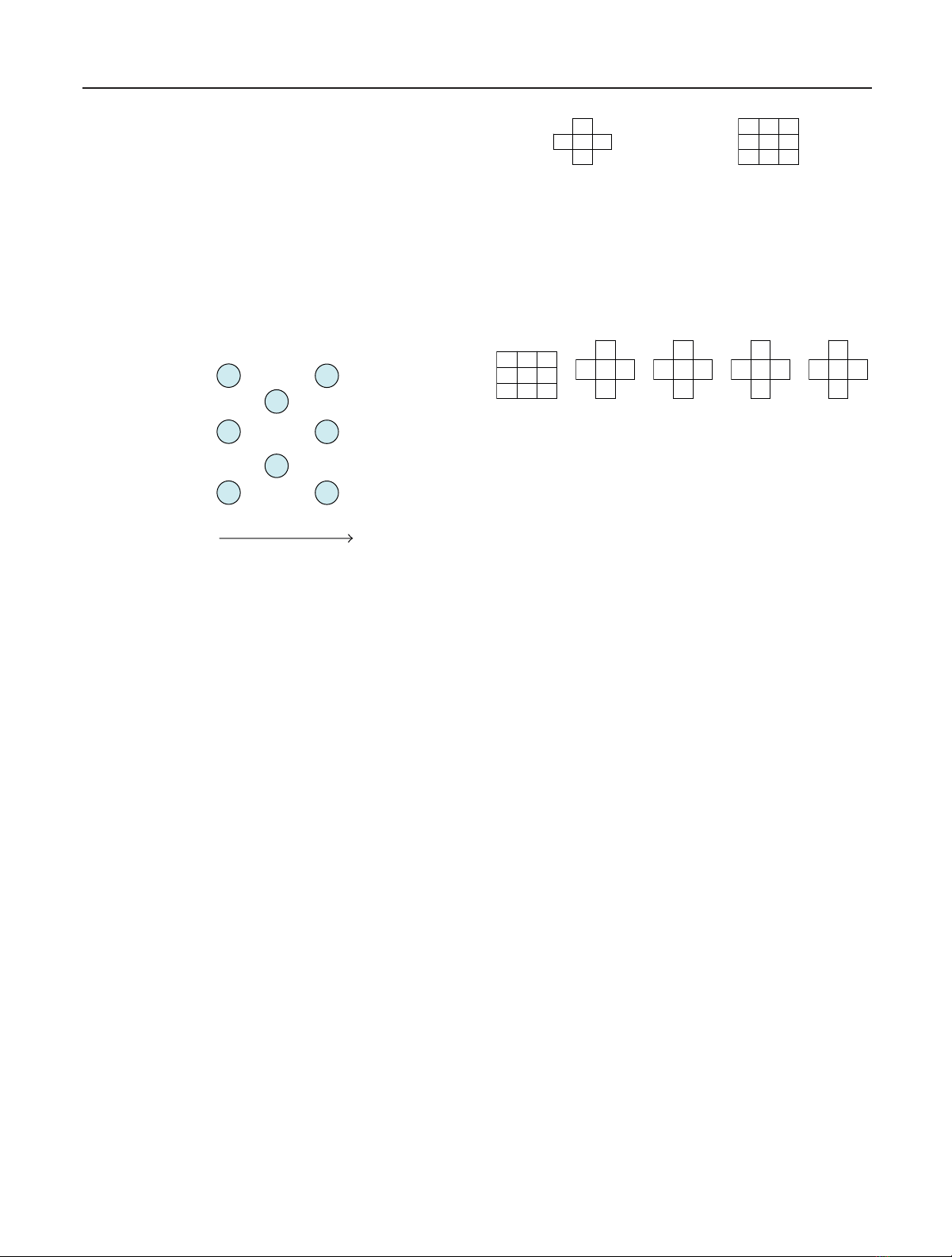
We employ a binary nonsymmetric opening morpholog-
ical filter to further refine the motion map of HMD. First,
an erosion filter with a cross-shaped mask, as shown in
Figure 3(a), is performed on the results of HMD. The ero-
sion filter eliminates isolated moving pixels. A dilation filter
with a 3 ×3 mask, as shown in Figure 3(b),isperformedaf-
ter erosion to restore and extend the shape of moving objects
after erosion. The inability to detect motion is referred to as
motion missing, which results in motion holes on the interpo-
lated images, and the detected motion of stationary objects as
false motion. The nonsymmetric opening morphological fil-
A
BXC
D
Erosion output at position
X=min(A,B,C,D,X)
(a) Erosion output at posi-
tion X =minimum (A, B, C,
D, X)
ABC
D
F
XE
GH
Dilation output at position
X=max(A,B,C,D,E,F,G,H,X)
(b) Dilation output at position X
=maximum (A, B, C, D, E, F, G,
H, X)
Figure 3: Nonsymmetric opening operation. (a) Erosion, (b) dila-
tion.
paq
b
r
Xc
ds
(a)
H
HXH
L
(b)
H
LXL
L
(c)
H
HX L
L
(d)
H
LXL
H
(e)
Figure 4: Edge pattern. (a) Pixel definition, (b) 3H1Lpattern, (c)
3L1Hpattern, (d) 2H2Lcorner pattern, (e) 2H2Lstripe pattern.
ter can minimize the visual artifact caused by motion missing
problem and enhance the overall performance in spite of the
corresponding false motion problem.
In our HMD, two filtering strategies, that is, the first and
the second conditions, are used to cover motion with vari-
ous speed and result in correct detection of motion. Mov-
ing edges are also considered by the third condition. The in-
clusive detection strategies contribute to the adaptability of
HMD. Moreover, the short field delay offers higher temporal
correlation for interpolation than 4-fileld and 5-field algo-
rithms. Its low-memory cost also makes it attractive for VLSI
implementation.
2.2. Interpolation
There are two interpolation schemes in the proposed
motion-adaptive deinterlacing algorithm to be chosen from.
EPR is the intra-field interpolator used in moving scenes, and
FI is the inter-field interpolator used in stationary scenes.
HMD adaptively selects intra-field or inter-field interpola-
tion as the output.
Moving textures are very difficult to interpolate because
aliasing may already exist after interlacing as explained by the
spectral analysis in [2]. Inspired by color filter array, which
has been widely used in cost-effective consumer digital still
cameras [19], we adapt it for texture and edge interpola-
tions. In Figure 4,therearefouruniquetypesofedgepat-
terns within a 3 ×3 window, which are 3H1Ledge patterns,
3L1Hedge patterns, 2H2Lcorner patterns, and 2H2Lstripe
patterns. The definition of “H”and“L” pixels is similar to
delta modulation in communications systems. If the pixel
value is larger than the average of pixel a,b,c,andd,itis
marked as “H”andmarkedas“L” otherwise. We can obtain
14 distinct patterns with different orientations.
By considering 3H1Land 3L1Hedge patterns in Figures
4(b) and 4(c), it is obvious that the center pixel Xis very
likely to be one of the majority neighbor pixels. Hence, the
4 EURASIP Journal on Image and Video Processing
pHq
H
r
XL
Ls
if |p−q|>|r−s|
X←− min(H,H)
else
X←− max(L,L)
pHq
H
r
HL
Ls
pHq
H
r
LL
Ls
Figure 5: The interpolation method of 2H2Lcorner pattern.
pHq
L
r
XL
Hs
if |p−q|+|r−s|>|p−r|+|q−s|
X←− min(H,H)
else
X←− max(L,L)
pHq
L
r
HL
Hs
pHq
L
r
LL
Hs
Figure 6: The interpolation method of 2H2Lstripe pattern.
median of Hor Lpixels around Xare calculated as the in-
terpolation result. Consider the 2H2Lcorner pattern shown
in Figure 4(d), the gradients in horizontal directions, |p−q|
and |r−s|,arecomputed.If|p−q|is larger than |r−s|,it
indicates that the gradient at upper position is larger than
that at lower position. There is an “H” corner in the 3 ×
3 window. In this condition, the function minimum(H,H)
is applied to interpolate pixel X; Otherwise, there is a “L”
corner and the function maximum(L,L) is applied as shown
in Figure 5. The other three corner patterns can be calcu-
lated in a similar way. As for the 2H2Lstripe pattern in
Figure 4(e), four gradient values, |p−q|,|r−s|,|p−r|,
and |q−s|are computed here. As shown in Figure 6, if the
sum of horizontal gradient values is larger than the sum of
vertical ones, minimum(H,H) is applied because there ex-
ists a vertical edge; otherwise, the function maximum(L,L)
is used due to a horizontal edge. The median filter of 3H1L
and 3L1Hpatterns, and the minimum filter and maximum
filter of “H” pixels and “L” pixels can avoid the interpolation
of an extreme value and thus minimize the risk of “pepper &
salt” noises.
The pixels band cin Figure 4(a),likeX, are also missing
pixels in interlaced video. To prevent error propagation, we
adaptively obtain bfrom the previous field if it is detected
as stationary and from the average of pand rif it is mov-
ing. Likewise, the value of ccan be calculated for EPR of X.
Predicting band cadaptively from either spatial or tempo-
ral neighbors greatly increases their correlation with the X,
which again helps with the pattern analysis and interpola-
tion.
EPR provides a low-complexity deinterlacer which effi-
ciently adapts to textural and edge contents during interpo-
Table 1: The abbreviations of the algorithms.
Abbreviation Full name
FI Field-insertion
LA Line-average
ELA Edge-based line-average [3]
EELA Enhanced edge-based line-average [5]
EPR Edge-pattern recognition (proposed)
HMD Hybrid motion detection (proposed)
HMDEPR Motion-adaptive deinterlacing with HMD
and EPR (proposed)
2FMA 2-field motion-adaptive deinterlacing
3FMA 3-field motion-adaptive deinterlacing
4FTD 4-field motion-adaptive algorithm with
texture detection [21]
4FHMD 4-field motion-adaptive algorithm with
horizontal motion detection [5]
lation. The uniqueness in using EPR in deinterlacing is that
complex scenes with textures or edges are analyzed and cate-
gorized into reasonable number of patterns by delta modula-
tion, which adaptively determines on the prediction value for
the one-bit encoding of the four pixels and thus accommo-
dates extensive cases of input video. The pattern encoding is
followed by an associated filtering scheme using the contex-
tual information from the vicinity having high correlation.
The simple hardware realization of delta modulation and the
corresponding operations also makes EPR more favorable.
3. EXPERIMENTS AND THE RESULTS
Deinterlacing is commonly applied to standard definition
(SD) video signals such as PAL and NTSC. We have experi-
mented on several SD video sequences for subjective compar-
ison. However, to objectively and comprehensively present
the performance of HMDEPR, we also show the results of
CIF video sequences. When the same continuous video sig-
nal is sampled in CIF and SD resolution, the CIF sequence
would have a wider spectrum and have more high-frequency
components near the interlace replicas than SD after inter-
lacing [2,20]. The CIF sequences are thus used as critical test
conditions.
We compared our algorithm to LA, FI, 2-field motion-
adaptive algorithm (2FMA), 3-field motion-adaptive algo-
rithm (3FMA), 4-field motion-adaptive algorithm with tex-
ture detection (4FTD) [21], and 4-field motion-adaptive al-
gorithm with horizontal motion detection (4FHMD) [5].
To facilitate the reading, we summarize the abbreviation of
these algorithms in Table 1. The detailed setting of all al-
gorithms and other experimental conditions are described
in Section 3.1. To clearly demonstrate the performance of
our algorithm, we separate the experiments into three parts.
Section 3.2 analyzes our motion-detection algorithm with
the contribution of each step. The second part, shown in
Section 3.3, compares the EPR algorithm with other intra-
interpolation methods. In Section 3.4,wecombineFI,EPR,
Gwo Giun Lee et al. 5
if abs(pi(i,j−1, k)−pi(i,j,k−1)) >TH2FMD
line-average,
else
field-insertion,
Algorithm 1
if abs(pi(i,j,k−1) −pi(i,j,k+1))>TH2FMD
line-average,
else
field-insertion.
Algorithm 2
and HMD as the deinterlacer and show its subjective and ob-
jective performance and comparison.
3.1. Experimental settings
2FMA and 3FMA are two simple motion-adaptive algo-
rithms used to highlight the accuracy of HMDEPR. The de-
tail of 2FMA is described as in Algorithm 1 where the sym-
bolic definition is the same as in 1.
3FMA, also known as the simplest same-parity motion
detection, is described as in Algorithm 2.
4FTD [21] performs not only motion detection, but also
texture detection. The simplified algorithm is described as
in Algorithm 3 where max diffis the maximum of three ab-
solute differences in the 4-field motion detection. Var is the
variance of the 3 ×3 spatial block centered at the current
pixel. This algorithm classifies the current pixel as one of
the four cases: moving textural region, moving smooth re-
gion, static textural region, and static smooth region with
associated interpolation methods. The pixels used in 3-
dimensional (3D) ELA in [21] are missing pixels. In our ex-
periment, we reasonably use
pi(i+m,j+n,k+l)|m∈{−1, 0, 1},
n∈{−2, 2},l∈{−1, 1}.(2)
4FHMD [5] performs horizontal motion detection. If the
temporal difference is smaller than an adaptive threshold,
temporal interpolation along the moving direction will be
adopted. Otherwise, 5-tap EELA will apply to the motion
scenes. In the EELA, the threshold THEELA is required to en-
sure a dominate edge and thus avoid “pepper & salt” noises
caused by edge misjudgments. The current pixel for thresh-
old adjustment is missing, which is not explained in [5]. We
use the line average result for threshold adjustment in our
implementation.
Tabl e 2 shows the thresholds used throughout our exper-
iments. They are tuned to achieve optimally subjective and
objective output video quality. The threshold TH1 of our al-
gorithm is set to a small value to prevent motion missing
problem. Although it causes more false motion at the same
if max diff≥TH4FTD Motion,
AND Var >TH4FTD Te x tur e
3D −ELA,
else if max diff<TH4FTD Motion,
AND Var >TH4FTD Te x t ure
modified-ELA,
else if max diff≥TH4FTD Motion,
AND Var ≤TH4FTD Te x t ure
VT-linear-filter,
else
VT-median-filter,
Algorithm 3
time, this negative effect is alleviated by EPR. TH2 is set to
prevent erroneous opposite-parity difference that appears in
textural scenes. TH3 is set as the double of TH1, since two
difference pairs are involved. Quantitatively, the performance
is not sensitive to any thresholds in Table 2 since the PSNR
difference of the test sequences is less than 0.01 dB if we in-
crease or decrease one of the thresholds by one. Moreover,
the visual difference of changing TH1 from 4 to 12 is not
perceivable unless very carefully inspected.
In the determination of 2FMA, a large threshold favors
stationary scenes such as Silent and Mother & daughter,
while a small threshold benefits moving scenes. The value
was fixed to balance the gain and loss of all sequences. Similar
tradeoffwas made for the other thresholds. There was, how-
ever, a special situation in determining TH4FTD Texture.“Pep-
per & salt” noises are a serious problem in 3D ELA. Eventu-
ally, TH4FTD Texture was set to a large value to prevent choosing
3D ELA. Only sharp edges are detected as texture regions.
The PSNR of the kth frame is calculated by 5, where pp
is the pixel in progressive sequences. Mand Nare the frame
width and frame height. Other symbolic definitions are the
same as in 1. We exclude the boundary cases, the first and the
last line, in PSNR calculation. The PSNR in Section 3.4 is the
average value of all frames between the third frame and the F
−1th frame, where Fis the total frame number of a sequence:
PSNR(k)
=10 log10
2552
M−1
i=0N−2
j=1po(i,j,k)−pp(i,j,k)2/MN .
(3)
3.2. Experimental results of motion detection
We take the 157th motion map of foreman in CIF resolution
as an example to explain the contribution of HMD step-by-
step. In Figures 7(a)–7(f), the fused 156th and 157th fields
of Foreman are overlaid with motion maps. The transpar-
ent regions are the motion regions, and the opaque regions
are detected as stationary. The edges of the building and the
fast moving gesture are two crucial parts in motion detection,
since severe line crawl will be observed if the motion is not
detected correctly. All the regions with moving hand, either


%20--%3e%3cdefs%3e%3cstyle%3e%20.st0%20{%20fill:%20%23fff;%20}%20.st1%20{%20fill:%20%237800fa;%20}%20%3c/style%3e%3c/defs%3e%3cpath%20class='st1'%20d='M117.78,12.18H43.11c2.9,3.47,4.65,7.94,4.65,12.82,0,5.6-2.3,10.66-6.01,14.29h76.02l7.22-13.56-7.22-13.56Z'/%3e%3cg%3e%3cpath%20class='st0'%20d='M53.58,26.17h-.59v-1.46h.59v-4.96h2.83c1.78,0,2.67.94,2.67,2.82v5.76c0,1.87-.89,2.81-2.67,2.81h-2.83v-4.96ZM55.36,21.37v3.34h1.1v1.46h-1.1v3.34h1.01c.61,0,.91-.37.91-1.1v-5.93c0-.74-.3-1.1-.91-1.1h-1.01Z'/%3e%3cpath%20class='st0'%20d='M65.99,31.14h-1.8l-.31-2.07h-2.19l-.31,2.07h-1.64l1.82-11.39h2.62l1.82,11.39ZM65.28,18.04c-.25.46-.51.77-.75.94-.21.15-.47.22-.79.22-.26,0-.57-.07-.92-.22l-.38-.15c-.14-.05-.26-.07-.37-.07-.3,0-.53.18-.71.54l-.91-.68c.25-.46.51-.77.75-.94.21-.14.48-.21.79-.21.26,0,.57.07.92.21l.38.15c.14.05.26.07.37.07.3,0,.53-.18.71-.54l.91.68ZM61.91,27.52h1.73l-.87-5.76-.87,5.76Z'/%3e%3cpath%20class='st0'%20d='M74.53,26.89v1.52c0,1.91-.89,2.86-2.67,2.86s-2.67-.95-2.67-2.86v-5.93c0-1.91.89-2.86,2.67-2.86s2.67.95,2.67,2.86v1.11h-1.69v-1.22c0-.75-.31-1.12-.93-1.12s-.93.37-.93,1.12v6.15c0,.74.31,1.11.93,1.11s.93-.37.93-1.11v-1.63h1.69Z'/%3e%3cpath%20class='st0'%20d='M81.4,31.14h-1.8l-.31-2.07h-2.19l-.31,2.07h-1.64l1.82-11.39h2.62l1.82,11.39ZM75.9,19.2l1.52-1.91h1.71l1.51,1.91h-1.61l-.76-.95-.75.95h-1.61ZM77.32,27.52h1.73l-.87-5.76-.87,5.76ZM83.1,15.99l-1.76,1.91h-1.26l1.17-1.91h1.86Z'/%3e%3cpath%20class='st0'%20d='M84.86,19.75c1.78,0,2.67.94,2.67,2.82v1.48c0,1.87-.89,2.81-2.67,2.81h-.85v4.28h-1.79v-11.39h2.64ZM84.01,21.37v3.86h.85c.58,0,.87-.36.87-1.08v-1.71c0-.71-.29-1.07-.87-1.07h-.85Z'/%3e%3cpath%20class='st0'%20d='M93.51,19.75c1.78,0,2.67.94,2.67,2.82v1.48c0,1.87-.89,2.81-2.67,2.81h-.85v4.28h-1.79v-11.39h2.64ZM92.66,21.37v3.86h.85c.58,0,.87-.36.87-1.08v-1.71c0-.71-.29-1.07-.87-1.07h-.85Z'/%3e%3cpath%20class='st0'%20d='M98.8,31.14h-1.79v-11.39h1.79v4.88h2.03v-4.88h1.83v11.39h-1.83v-4.88h-2.03v4.88Z'/%3e%3cpath%20class='st0'%20d='M105.36,24.55h2.46v1.62h-2.46v3.34h3.09v1.63h-4.88v-11.39h4.88v1.63h-3.09v3.18ZM108.17,17.29l-1.76,1.91h-1.26l1.17-1.91h1.86Z'/%3e%3cpath%20class='st0'%20d='M112.2,19.75c1.78,0,2.67.94,2.67,2.82v1.48c0,1.87-.89,2.81-2.67,2.81h-.85v4.28h-1.79v-11.39h2.64ZM111.35,21.37v3.86h.85c.58,0,.87-.36.87-1.08v-1.71c0-.71-.29-1.07-.87-1.07h-.85Z'/%3e%3c/g%3e%3ccircle%20class='st1'%20cx='25'%20cy='25'%20r='20'/%3e%3cpath%20class='st0'%20d='M32.78,19.27c2.92,0,4.43,2.55,5.28,5.33l.71,2.17c.14.38-.33.75-.71.75h-5.61c.19-.33.24-.71.09-1.08l-.75-2.45c-.43-1.32-.99-2.64-1.79-3.77.75-.57,1.65-.94,2.78-.94h0ZM25,18.38c3.25,0,4.9,2.78,5.89,5.89l.76,2.45c.14.42-.33.8-.8.8h-11.69c-.42,0-.94-.38-.8-.8l.75-2.45c.99-3.11,2.64-5.89,5.89-5.89h0ZM25,11.35c1.74,0,3.11,1.37,3.11,3.11s-1.37,3.11-3.11,3.11-3.11-1.41-3.11-3.11,1.41-3.11,3.11-3.11h0ZM17.27,19.27c1.08,0,1.98.38,2.73.94-.8,1.13-1.37,2.45-1.74,3.77l-.8,2.45c-.14.38-.05.75.09,1.08h-5.56c-.42,0-.9-.38-.75-.75l.71-2.17c.9-2.78,2.41-5.33,5.33-5.33h0ZM17.27,12.91c1.51,0,2.78,1.27,2.78,2.83s-1.27,2.83-2.78,2.83-2.83-1.27-2.83-2.83,1.27-2.83,2.83-2.83h0ZM32.78,12.91c1.56,0,2.78,1.27,2.78,2.83s-1.23,2.83-2.78,2.83-2.83-1.27-2.83-2.83,1.27-2.83,2.83-2.83h0ZM27.07,28.56v.09c0,.57-.24,1.08-.61,1.46h0v.05c-.38.33-.9.57-1.46.57s-1.08-.24-1.46-.61h0c-.38-.38-.61-.9-.61-1.46v-.09h1.41v.09c0,.19.05.38.19.47v.05c.09.09.28.19.47.19s.38-.09.47-.19v-.05c.14-.09.24-.28.24-.47t-.05-.09h1.41ZM30.99,28.56v.09c0,1.65-.66,3.16-1.74,4.24-1.08,1.08-2.59,1.79-4.24,1.79s-3.16-.71-4.24-1.79l-.05-.05c-1.04-1.08-1.7-2.55-1.7-4.2v-.09h1.41v.09c0,1.27.47,2.4,1.27,3.25h.05c.85.85,1.98,1.37,3.25,1.37s2.4-.52,3.25-1.37c.85-.8,1.37-1.98,1.37-3.25v-.09h1.37ZM34.99,28.56v.09c0,2.78-1.13,5.28-2.92,7.07-1.79,1.79-4.29,2.92-7.07,2.92s-5.23-1.13-7.07-2.92c-1.79-1.79-2.92-4.29-2.92-7.07v-.09h1.41v.09c0,2.4.94,4.53,2.5,6.08,1.56,1.56,3.72,2.5,6.08,2.5s4.52-.94,6.08-2.5c1.56-1.56,2.5-3.68,2.5-6.08v-.09h1.41Z'/%3e%3c/svg%3e)