
Hindawi Publishing Corporation
EURASIP Journal on Advances in Signal Processing
Volume 2009, Article ID 467549, 10 pages
doi:10.1155/2009/467549
Research Article
Automatic Evaluation of Landmarks for
Image-Based Navigation Update
Stefan Lang and Michael Kirchhof
FGAN-FOM Research Institute for Optronics and Pattern Recognition, Gutleuthaußtr. 1, 76275 Ettlingen, Germany
Correspondence should be addressed to Michael Kirchhof, kirchhof@fom.fgan.de
Received 29 July 2008; Revised 19 December 2008; Accepted 26 March 2009
Recommended by Fredrik Gustafsson
The successful mission of an autonomous airborne system like an unmanned aerial vehicle (UAV) strongly depends on its accurate
navigation. While GPS is not always available and pose estimation based solely on Inertial Measurement Unit (IMU) drifts,
image-based navigation may become a cheap and robust additional pose measurement device. For the actual navigation update
a landmark-based approach is used. It is essential that the used landmarks are well chosen. Therefore we introduce an approach
for evaluating landmarks in terms of the matching distance, which is the maximum misplacement in the position of the landmark
that can be corrected. We validate the evaluations with our 3D reconstruction system working on data captured from a helicopter.
Copyright © 2009 S. Lang and M. Kirchhof. This is an open access article distributed under the Creative Commons Attribution
License, which permits unrestricted use, distribution, and reproduction in any medium, provided the original work is properly
cited.
1. Introduction
Autonomous navigation is of growing interest in science as
well as in industry. The key problem of most existing outdoor
systems is the dependency on GPS data. Since GPS is not
always available we integrate an image-based approach into
the system. Landmarks are used to update the actual position
and orientation. Thus it is necessary to select the landmarks
carefully. This selection takes place in an offline phase before
the mission. The evaluation of these landmarks is the main
contribution of this paper. For the online phase, we compute
3D reconstructions from the scene and match them with the
selected georeferenced landmarks.
In our terms a landmark is a subset of a point cloud
consisting of highly accurate LiDAR data.
There are already some systems that rely on image-
based navigation by recognition of landmarks. At present
all landmarks are manually selected by a human supervisor.
We address the question if this is the optimal solution.
The question arises since a human does the recognition or
registration of the data due to very high level features while
the system that has to deal with the landmarks operates on
similarities on low level features such as the 3D point cloud.
The proposed automatic evaluation of landmarks in
terms of matching distance (or convergence radius) enables
us to select the density of the landmarks in a manner that
assures that even in the presence of IMU drift (which can be
predicted from the previous measurements) the landmarks
can still be recognized by the system.
The matching distance (or convergence radius), which is
used in our evaluation method, is the maximum misplace-
ment of the position of a landmark, that can be corrected.
Thus it is a measure of the robustness of the considered
landmark.
Scene reconstruction and (relative) pose estimation are
very important tasks in photogrammetry and computer
vision. Some typical solutions are given in [1–5]. While
Akbarzadeh et al. [1]andNist
´
er et al. [5]workwitha
camera system with at least two cameras with known relative
position, they are able to determine the exact scale. In
contrast the solutions in [2–4,6]areonlydefinedupto
scale. In addition [6] evaluates the positioning problem in
terms of occlusion, speed, and robustness. Our work is based
on [7] where the 3D reconstrction is computed by feature
tracking [8] and triangulation [9] from known camera
positions.
The advantage of this method is that with the (approxi-
mately) given camera positions the resulting reconstruction
has an exact scale. Therefore the reconstruction and pose
estimation are only biased—by the drift of the Inertial
2 EURASIP Journal on Advances in Signal Processing
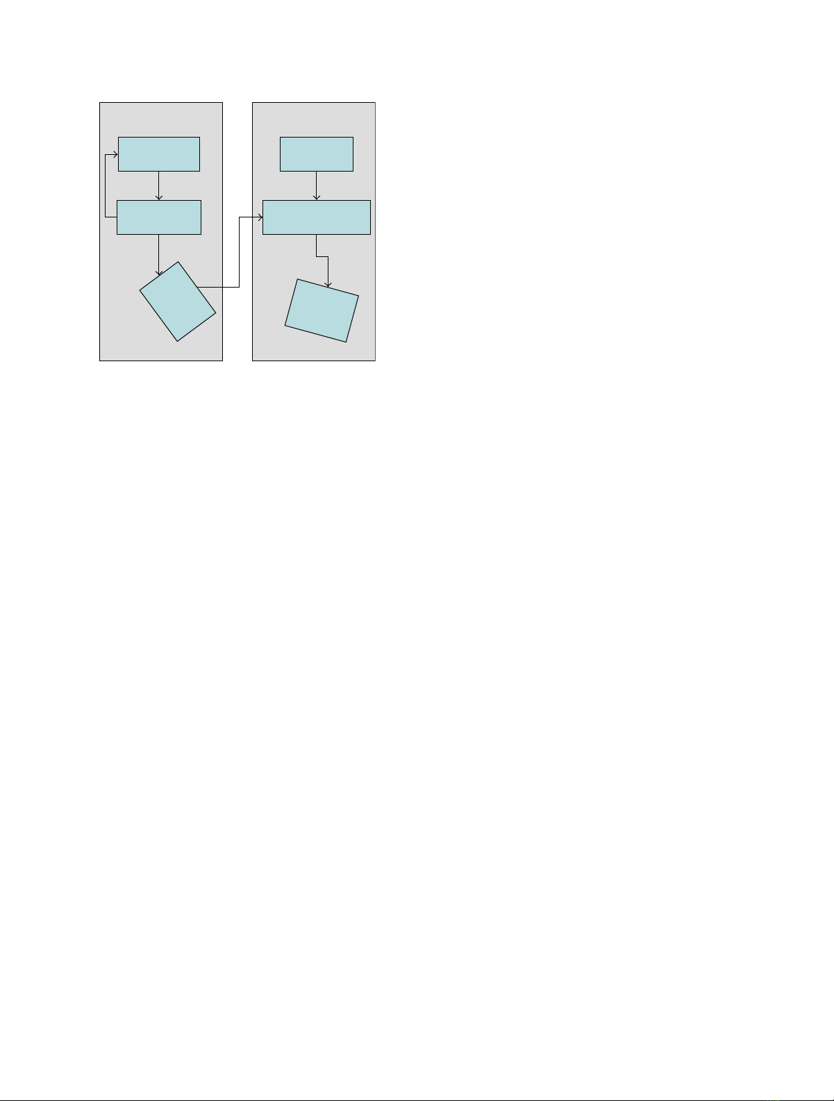
Online phaseOffline phase
Evaluation of
landmarks
Fusion and
path planning
Structure
from motion
Image based
navigation update
Landmark
Final
landmark
position
Figure 1: Overview of our landmark-based navigation system.
In the offline phase before the mission landmarks are evaluated
and fused with the path planning. During the online phase the
navigation data are updated by mean of the registation of the
landmarks with the SfM point cloud.
Navigation System (INS) or in absence of GPS of the IMU
alone—resulting in fewer parameters in the registration
process, which is based on Iterative Closest Point (ICP) [10]
in our approach. Reference [11] showed an application of
ICP-based registration of continuous video onto 3D point
clouds for optimizing the texture of the point cloud. A
different solution to the registration that is not adressed here
is described in [6]. Lerner et al. [12]provideasolution
to pose and motion estimation based on registration with
a Digital Terain Model (DTM). While saving the DTM
for the complete flight path is critical we focus on the
selection of “good” landmarks. For pedestrians and cars
some evaluations of landmarks had been done in terms
of permanence, uniqueness, and visibility [13–17]. In our
context uniqueness and matching distance are the most
relevant factors.
Our paper is organized as follows. The second part
of the paper describes the different methodologies used
throughout the paper. The focus is on the evaluation of
landmarks, which is described first. Path planning by means
of given landmarks, a simple approach for 3D-reconstruction
and an approach to image-based navigation update are
outlined as part of the complete system. In the following
part experiments, first the experimental setup and used
data sets are presented. Then we give the results of the
evaluation of several landmarks. Additionally results of tests
of the complete system are shown. The paper closes with a
discussion and conclusion.
2. Methodology
It is assumed that highly accurate 3D data of an area are
given. A landmark will be called optimal if the probability
to recover it in the later mission is maximal. For that purpose
meaningful measures for evaluation of landmarks have to be
developed.
In contrast to simply defining a cost function for
evaluation of a landmark, the method to find the landmark
is used directly for evaluation. As further requirement the
rotation and translation which align the reconstructed area
with the found landmark are needed. For that purpose the
ICP method [10] is used, which is a standard approach for
registering two point clouds.
The evaluation and thus the selection of landmarks will
take place in an offline phase before the mission. In this phase
all given information are fused and the path planned. Then
during mission in the online phase, both the reconstructed
point cloud, obtained by the SfM system, and the landmarks
are registered and the final landmark position estimated.
The calculated transformation information can be used for
an image-based navigation update. The whole system is
presented in Figure 1.
2.1. Evaluation of Landmarks. A landmark given by many
highly accurate 3D points will be evaluated by means of all
available information. Considering the functionality of the
used ICP, the following design issues are important.
(i) Size and structure of the landmark.
(ii) Structure of the local area surrounding the landmark.
(iii) Uniqueness of the landmark in the wider considered
area.
These issues led to a combination of a local and a global
evaluations. The local evaluation fulfills the constraints in
taking the size and structure of the landmark as well as the
structure of the surrounding area into account. A house in a
highly cluttered area is not a very meaningful landmark since
ICP would not be able to retrieve the exact orientation of the
landmark and thus should get a bad evaluation. The third
constrain, the uniqueness of the landmark in the considered
area, needs a global view on the area. Objects similar to
the tested landmark, which could lead to confusion in the
recovery process have to be detected and therefore should
receive a bad evaluation result. For example a house next to
a similar house is not a very meaningful landmark and thus
should get a bad evaluation.
2.1.1. Local Evaluation. Let Dlandmark be a set of 3D points
describing a landmark and let Darea be a set of 3D points
defining the given area. If there is an error in the estimated
pose of the observer, the area will be rotated and translated.
Thus the coordinate system is first rotated around the center
of the landmark with Rand then shifted by t. The rotation
matrix Ris constructed as follows:
R=
⎛
⎜
⎜
⎝
cos(θz)−sin(θz)0
sin(θz)cos(θz)0
001
⎞
⎟
⎟
⎠,(1)
where θzis the rotation angle around the z-axis. The changes
in the 3D points p∈R3of Darea can be calculated with
D′
area =p′|p′=Rp +t,p∈Darea.(2)

EURASIP Journal on Advances in Signal Processing 3
Input parameters: Dlandmark,Darea,dx,dy,θmax
1: for all −θmax ≤θz≤θmax do
2: for all −dy≤y≤dydo
3: for all −dx≤x≤dxdo
4: t←(x,y,0)
T
5: R←euler2rot(θz)
6: D′
area ←{p′|p′=Rp +t,p∈Darea}
7: Rcalc,tcalc ←ICP(D′
area,Dlandmark)
8: ǫt(x,y)←t−tcalc
9: ǫθ(x,y)←|θz−rot2eulerz(Rcalc)|
10: end for
11: end for
12: end for
Algorithm 1: Landmark grid test method.
For the evaluation a landmark is tested for different
translations and rotations. As already mentioned in (1)we
ignore rotations and translations that effect the ground plane
(z=0) for reducing the complexity of the simulation.
The previous experiments showed that these parameters can
be ignored because ICP always registered the ground plane
correct, because all the data expand along this plane.
In each cycle the ICP algorithm is performed with D′
area
and Dlandmark. For later evaluation the position error ǫt(x,y)
and rotation error ǫθ(x,y) in a grid around the landmark
position and different angles are calculated. Algorithm 1
shows the implementation of this “Landmark Grid Test
Method.” The algorithm iterates over all angles and grid
points given by the input parameters. The used methods
euler2rot and rot2euler convert a rotation angle to a rotation
matrixandviceversa.Asmainfunctioncall,seestep7,
the method ICP calculates the transformation parameters
aligning D′
area with Dlandmark.
For each applied angle θz∈[−θmax,θmax] the error
images ǫtand ǫθare obtained. These slices contain errors
with respect to translation and rotation for each grid point.
They are converted by means of defined thresholds for
maximum allowed translation and rotation error. The results
are binary images with the entry one where the method
converged to the right result and zero otherwise. The sum of
all ones in each slice is used as a measure for the evaluation
and comparison of the landmarks. Additionally vectors to the
minimum and maximum grid points with a value one are
used in the evaluation of the landmarks, too. These vectors
are depicted in the second row of Figure 9.Appartfrom
the evaluation measure they define a minimal and maximal
matching distance which is required for the path planning.
While the minimal matching distance is equivalent to the
radius of convergence, the maximum matching distance is
the largest distance from which the ICP converged against
the solution.
2.1.2. Global Evaluation. In global consideration a landmark
will be evaluated by means of the whole area. For that
purpose a binary mask of the area is generated, by projecting
the 3D points to an image plane parallel to (z=0) with a
pixel size of 10 by 10 meters. The entries of this image are
one if there is at least one 3D points projected to the pixel
otherwise zero. Next, the binary image is preprocessed for
our purposes by means of morphological operations. First
the operation closing is performed to fill holes (zeros) in the
mask of the area. Then the mask is eroded with a mask of
the landmark as structured element to avoid the border of
the area. The different steps of this approach are shown in
Figure 2.
For each entry of the mask equal one, the landmark is
moved to the corresponding position in the area but not
rotated and the ICP method is applied. The result is assigned
to that position. With this described approach local minima
with respect to the ICP’s cost function can be spotted. The
global minimum is expected to be at the center of the origin
landmark position.
Considering that the ICP error function erficp is a sum
of least squares, the error function is equivalent to the
Log-Likelihood function describing the probability that the
data are an instance of the model. The original likelihood
is a natural measure for the instances. Assuming that ICP
converges towards the global minimum Xglobalmin (ground
truth) or the second smallest local minimum Xlocalmin the
probability for matching the model with the ground truth
is given by
G=e−erficp (Xglobalmin)
e−erficp (Xglobalmin)+e−erficp(Xlocalmin ).(3)
Indeed this measure depends on the precision of the data. But
assuming that all the derived 3D points have approximately
the same deviation (approximately one) there is just a linear
scaling between the likelihood and the probability which is
approximately compensated by the denominator in (3). The
normalization leads to the codomain [0, 1).
2.2. Fusion and Path Planning. When selecting landmarks
for navigation the first problem one has to address is the
uniqueness of the landmarks. A measure for the uniqueness
is the discriminatory power of the landmarks to local minima
during the ICP/registration process. In the absence of the
absolute probabilities, randomly chosen landmarks within a
search region are first sorted by the global measure (3)which
corresponds to the discriminatory power. The best 20% of
the landmarks are treated further with the local evaluation.
The local evaluation gives a measure for the volume
of the parameter space from which ICP converges against
the ground truth. Therefore it is related to the speed of
convergence and the radius of convergence. Within the local
evaluation one can compute the smallest distance of the
surface to the reference position. This distance describes the
precision that the UAV should have during approaching the
landmark. Knowing the drift of the UAV one can define the
search region for the next landmark.
The resulting path planning algorithms work as follows.
Starting from the target landmark one measures the smallest
radius of convergence. The prediction of the system’s drift
(known from IMU specification) defines a region for the
preceding landmark. This region is sampled with manually
4 EURASIP Journal on Advances in Signal Processing
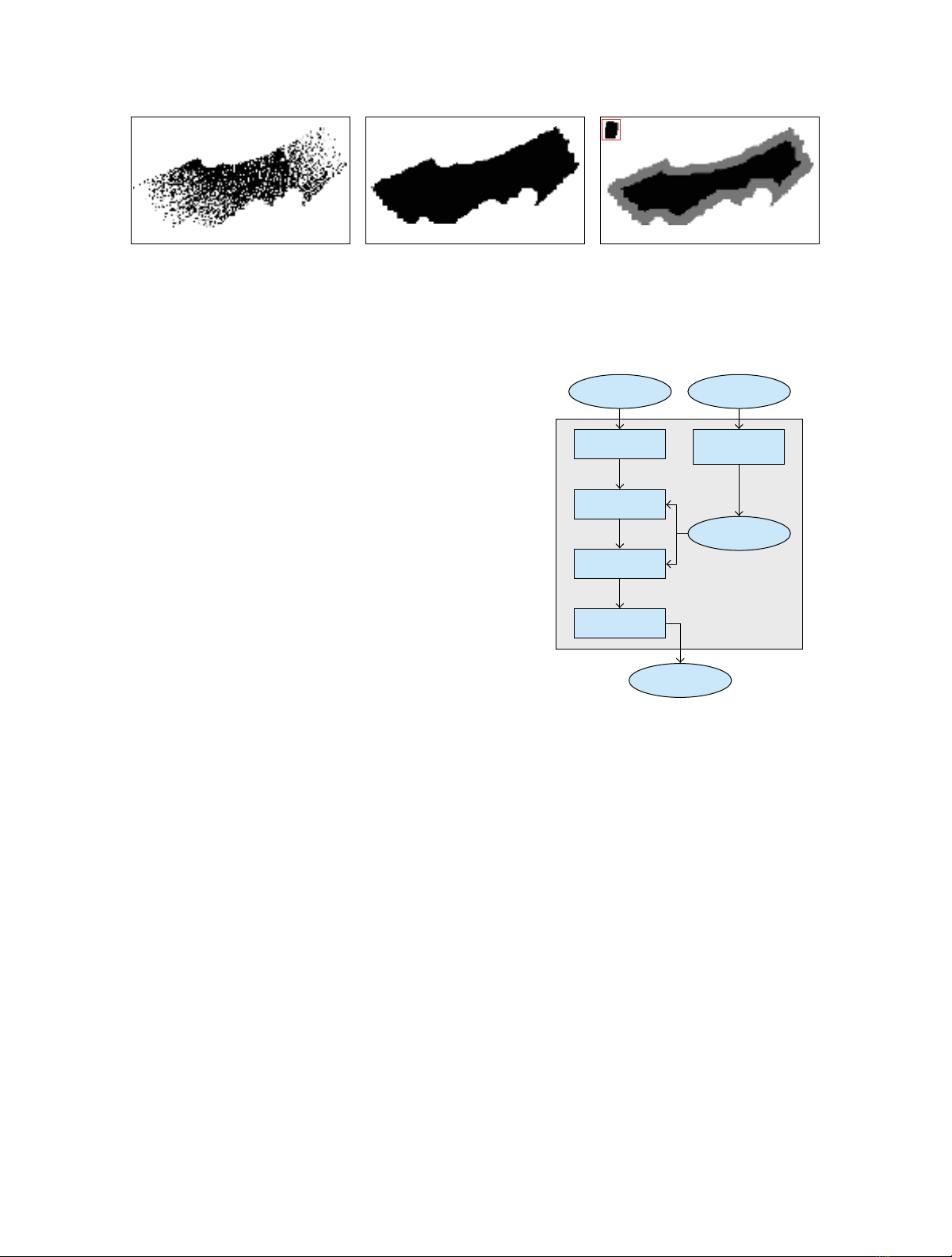
(a) (b) (c)
Figure 2: Creation of the binary mask for the tests. (a) Initialized mask with black pixels if a 3D laser point is found in the defined
neighborhood. (b) Mask after the closing operation. (c) The gray area is eroded by means of a mask of the landmark as structured element
(upper left, red box). The final mask consists of the residual black pixels.
or randomly chosen landmarks. These landmarks are then
evaluated with the methods described in Sections 2.1.1 and
2.1.2 resulting in a decision for the best landmark. This
method is repeated until one reaches the starting point of the
UAV.
2.3. Structure from Motion/3D Reconstruction. In this section
the Structure from Motion (SfM) system to calculate a
3D point cloud from given IR images is described briefly.
Additionally the approach using orientation and position
information of the sensor to obtain more accuracy in the
reconstruction is described. The implementation is based on
Intel’s computer vision library OpenCV [18].
A system overview is given in Figure 3. After initializa-
tion, detected features are tracked image by image. In order
to minimize the number of mismatches between the corre-
sponding features in two consecutive images the algorithm
checks the epipolar constraint by means of the given pose
information retrieved from the INS. Triangulation of the
tracked features results in the 3D points. Each 3D point
is assessed with the aid of its covariance matrix which is
associated with the respective uncertainty. Finally a nonlinear
optimization yields the completed point cloud.
The modules are described in more detail in the following
sections.
2.3.1. Tracking Features. To estimate the motion between
two consecutive images the OpenCV version [19] of the
KLT tracker [8] is used. The algorithm tracks corners or
corner-like point features. For robust tracking a measure of
feature similarity is used. This weighted correlation function
quantifies the change of a tracked feature between the current
image and the image of initialization of the feature.
2.3.2. Retrieve Orientation and Position. TheINSgivesthe
Kalman-filtered [20] absolute position and orientation of the
reference coordinate frame. After converting the data into
absolute rotation matrices Rabs
iand position vectors
Cifor
the absolute orientation and position of the ith camera in
space, the projection matrices Pi, needed for triangulation,
are calculated as follows:
Pi=KRabs
iI3|−
Ci,(4)
where K is the intrinsic camera matrix and Pia3×4-matrix.
IR-images
Track features
Check features
Triangulate
Refine 3D points
3D point cloud
IMU/GPS
Pose/position
Retrieve pose
and position
Figure 3: Overview of the SfM modules. Features are tracked in
consecutive images and checked for satisfaction of the epipolar
constraint. Linear Triangulation of each track of the checked
features gives the 3D information. In both steps—constraint
checking and triangulation—the retrieved orientation and position
information is used. Finally each 3D point are evaluated and
optimized.
2.3.3. Epipolar Constraint. With the aid of the epipolar con-
straint mismatches in the feature tracking can be detected.
Both the relative rotation R and the relative translation t
between two consecutive images are given. As described in
[3] the fundamental matrix can be calculated according to
F=KT−1[t]×RK−1.(5)
With the skew-symmetric matrix [t]×of the vector t.To
check whether x′is the correct image point corresponding
to the tracked point feature xof the previous image, x′has to
lie on the epipolar line l′defined as
l′≡Fx.(6)
Normally a corresponding image point does not lie exactly
on the epipolar line, due to noise in the images and
inaccuracies in pose measures. Thus we allow for some
EURASIP Journal on Advances in Signal Processing 5
distance (error) of x′to l′. But we reject the feature if the
distance becomes too large and the track ends.
2.3.4. Triangulation. During iteration over the IR images,
tracks of detected and tracked point features are built and
the corresponding 3D point Xis calculated. In [9]agood
overview of different methods for triangulation is given as
well as a description of the method used in our system.
Let x1,...,xnbe the image features of the tracked 3D
point Xin nimages and P1,...,P
nthe projection matrices
of the corresponding cameras. Each measurement xiof the
track represents the reprojection of the same 3D point
xi≡PiXfor i=1, ...,n. (7)
With the cross-product the homogeneous scale factor of (7)
is eliminated, which leads to xi×(PiX)=0. Subsequently
there are two linearly independent equations for each image
point. These equations are linear in the components of X,
thus they can be written in the form AX=0, where A is the
corresponding action matrix [9].The3DpointXis the unit
singular vector corresponding to the smallest singular value
of the matrix A.
2.3.5. Nonlinear Optimization. After triangulation the repro-
jection error can be estimated as follows:
ǫi=⎛
⎝ǫx
i
ǫy
i
⎞
⎠=d(X,P
i,xi)=
⎛
⎜
⎜
⎜
⎜
⎝
xi−p1
iX
p3
iX
yi−p2
iX
p3
iX
⎞
⎟
⎟
⎟
⎟
⎠.(8)
With the assumption of a variance of the 2D position of one
pixel, the back-propagated covariance matrix of a 3D point
is calculated
ΣX=JTΣ−1
pJ−1.(9)
In this case the covariance of 2D position Σ−1
pequals the
2D identity matrix, with the Jacobian matrix J, which is the
partial derivative matrix ∂ǫ/∂X. The Euclidean norm of ΣX
gives an overall measure of the uncertainty of the 3D point X
and enables the algorithm to reject poor triangulation results.
With nonlinear optimization, a calculated 3D point can
be corrected. Using the Gauss-Newton method [21] yields
the corrected 3D points.
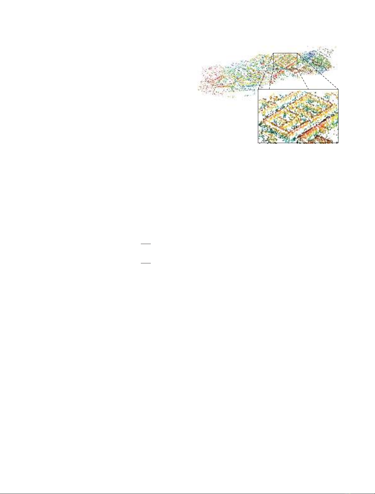
2.3.6. Results. Working on an IR sequence with 470 images
and taking orientation and position information into
account the system had calculated an optimized point cloud
of about 17 500 points see Figure 4. The height of each point
is coded in its color. Although it is a sparse reconstruction,
the structure of each building is well distinguishable and
there are only a few gross errors due to the performed
optimization.
2.4. Image-Based Navigation Update in the Complete System.
In the previous sections only highly accurate 3D points are
Figure 4: Calculated point cloud of an IR image sequence with
the magnification of one building. The overall number of points
is 17 606.
used for evaluation or selection of landmarks. That can be
considered as the preparation phase of a mission, where
LiDAR or other advanced sensors are used for measuring the
structure of the area.
The goal of the image-based navigation update is to
correct the INS drift with the help of the selected landmarks.
For this purpose the system descriped in Section 2.3 is used
to estimate a 3D point cloud on base of the INS poses
during the flight. Aligning this point cloud with the accurate
landmark models yields the transformation that is needed to
correct for the INS drift.
3. Experiments
3.1. Experimental Setup. As sensor platform a helicopter is
used. The different sensors are installed in a pivot-mounted
sensor carrier on the right side of the helicopter. The
following sensors are used.
IR camera. An AIM 640QMW is used to acquire midwave-
length (3–5 µm) infrared light. The lens has a focal
length of 28 mm and a field of view of 30.7◦×23.5◦.
LiDAR. The Riegl Laser Q560 is a 2D scanning device which
illuminates in azimuth and elevation with short laser
pulses. The distance is calculated based on the time of
flight of a pulse. It covers almost the same field of view
as the IR camera.
INS. The Inertial Navigation System (INS) is an Applanix
POS AV system which is specially designed for air-
borne usage. It consists of an IMU and a GPS system.
The measured orientation and position are Kalman-
filtered to smooth out errors in the GPS.
The range resolution of the LiDAR system is about 0.02 m
according to the specifications given by the manufacturer.
The absolute accuracy specifications of the Applanix system
state the following accuracies (RMS): position 4–6 m, veloc-
ity 0.05 m/s, roll and pitch 0.03◦, and true heading 0.1◦.


![Thuyết minh tính toán kết cấu đồ án Bê tông cốt thép 1: [Mô tả/Hướng dẫn/Chi tiết]](https://cdn.tailieu.vn/images/document/thumbnail/2016/20160531/quoccuong1992/135x160/1628195322.jpg)


%20--%3e%3cdefs%3e%3cstyle%3e%20.st0%20{%20fill:%20%23fff;%20}%20.st1%20{%20fill:%20%237800fa;%20}%20%3c/style%3e%3c/defs%3e%3cpath%20class='st1'%20d='M117.78,12.18H43.11c2.9,3.47,4.65,7.94,4.65,12.82,0,5.6-2.3,10.66-6.01,14.29h76.02l7.22-13.56-7.22-13.56Z'/%3e%3cg%3e%3cpath%20class='st0'%20d='M53.58,26.17h-.59v-1.46h.59v-4.96h2.83c1.78,0,2.67.94,2.67,2.82v5.76c0,1.87-.89,2.81-2.67,2.81h-2.83v-4.96ZM55.36,21.37v3.34h1.1v1.46h-1.1v3.34h1.01c.61,0,.91-.37.91-1.1v-5.93c0-.74-.3-1.1-.91-1.1h-1.01Z'/%3e%3cpath%20class='st0'%20d='M65.99,31.14h-1.8l-.31-2.07h-2.19l-.31,2.07h-1.64l1.82-11.39h2.62l1.82,11.39ZM65.28,18.04c-.25.46-.51.77-.75.94-.21.15-.47.22-.79.22-.26,0-.57-.07-.92-.22l-.38-.15c-.14-.05-.26-.07-.37-.07-.3,0-.53.18-.71.54l-.91-.68c.25-.46.51-.77.75-.94.21-.14.48-.21.79-.21.26,0,.57.07.92.21l.38.15c.14.05.26.07.37.07.3,0,.53-.18.71-.54l.91.68ZM61.91,27.52h1.73l-.87-5.76-.87,5.76Z'/%3e%3cpath%20class='st0'%20d='M74.53,26.89v1.52c0,1.91-.89,2.86-2.67,2.86s-2.67-.95-2.67-2.86v-5.93c0-1.91.89-2.86,2.67-2.86s2.67.95,2.67,2.86v1.11h-1.69v-1.22c0-.75-.31-1.12-.93-1.12s-.93.37-.93,1.12v6.15c0,.74.31,1.11.93,1.11s.93-.37.93-1.11v-1.63h1.69Z'/%3e%3cpath%20class='st0'%20d='M81.4,31.14h-1.8l-.31-2.07h-2.19l-.31,2.07h-1.64l1.82-11.39h2.62l1.82,11.39ZM75.9,19.2l1.52-1.91h1.71l1.51,1.91h-1.61l-.76-.95-.75.95h-1.61ZM77.32,27.52h1.73l-.87-5.76-.87,5.76ZM83.1,15.99l-1.76,1.91h-1.26l1.17-1.91h1.86Z'/%3e%3cpath%20class='st0'%20d='M84.86,19.75c1.78,0,2.67.94,2.67,2.82v1.48c0,1.87-.89,2.81-2.67,2.81h-.85v4.28h-1.79v-11.39h2.64ZM84.01,21.37v3.86h.85c.58,0,.87-.36.87-1.08v-1.71c0-.71-.29-1.07-.87-1.07h-.85Z'/%3e%3cpath%20class='st0'%20d='M93.51,19.75c1.78,0,2.67.94,2.67,2.82v1.48c0,1.87-.89,2.81-2.67,2.81h-.85v4.28h-1.79v-11.39h2.64ZM92.66,21.37v3.86h.85c.58,0,.87-.36.87-1.08v-1.71c0-.71-.29-1.07-.87-1.07h-.85Z'/%3e%3cpath%20class='st0'%20d='M98.8,31.14h-1.79v-11.39h1.79v4.88h2.03v-4.88h1.83v11.39h-1.83v-4.88h-2.03v4.88Z'/%3e%3cpath%20class='st0'%20d='M105.36,24.55h2.46v1.62h-2.46v3.34h3.09v1.63h-4.88v-11.39h4.88v1.63h-3.09v3.18ZM108.17,17.29l-1.76,1.91h-1.26l1.17-1.91h1.86Z'/%3e%3cpath%20class='st0'%20d='M112.2,19.75c1.78,0,2.67.94,2.67,2.82v1.48c0,1.87-.89,2.81-2.67,2.81h-.85v4.28h-1.79v-11.39h2.64ZM111.35,21.37v3.86h.85c.58,0,.87-.36.87-1.08v-1.71c0-.71-.29-1.07-.87-1.07h-.85Z'/%3e%3c/g%3e%3ccircle%20class='st1'%20cx='25'%20cy='25'%20r='20'/%3e%3cpath%20class='st0'%20d='M32.78,19.27c2.92,0,4.43,2.55,5.28,5.33l.71,2.17c.14.38-.33.75-.71.75h-5.61c.19-.33.24-.71.09-1.08l-.75-2.45c-.43-1.32-.99-2.64-1.79-3.77.75-.57,1.65-.94,2.78-.94h0ZM25,18.38c3.25,0,4.9,2.78,5.89,5.89l.76,2.45c.14.42-.33.8-.8.8h-11.69c-.42,0-.94-.38-.8-.8l.75-2.45c.99-3.11,2.64-5.89,5.89-5.89h0ZM25,11.35c1.74,0,3.11,1.37,3.11,3.11s-1.37,3.11-3.11,3.11-3.11-1.41-3.11-3.11,1.41-3.11,3.11-3.11h0ZM17.27,19.27c1.08,0,1.98.38,2.73.94-.8,1.13-1.37,2.45-1.74,3.77l-.8,2.45c-.14.38-.05.75.09,1.08h-5.56c-.42,0-.9-.38-.75-.75l.71-2.17c.9-2.78,2.41-5.33,5.33-5.33h0ZM17.27,12.91c1.51,0,2.78,1.27,2.78,2.83s-1.27,2.83-2.78,2.83-2.83-1.27-2.83-2.83,1.27-2.83,2.83-2.83h0ZM32.78,12.91c1.56,0,2.78,1.27,2.78,2.83s-1.23,2.83-2.78,2.83-2.83-1.27-2.83-2.83,1.27-2.83,2.83-2.83h0ZM27.07,28.56v.09c0,.57-.24,1.08-.61,1.46h0v.05c-.38.33-.9.57-1.46.57s-1.08-.24-1.46-.61h0c-.38-.38-.61-.9-.61-1.46v-.09h1.41v.09c0,.19.05.38.19.47v.05c.09.09.28.19.47.19s.38-.09.47-.19v-.05c.14-.09.24-.28.24-.47t-.05-.09h1.41ZM30.99,28.56v.09c0,1.65-.66,3.16-1.74,4.24-1.08,1.08-2.59,1.79-4.24,1.79s-3.16-.71-4.24-1.79l-.05-.05c-1.04-1.08-1.7-2.55-1.7-4.2v-.09h1.41v.09c0,1.27.47,2.4,1.27,3.25h.05c.85.85,1.98,1.37,3.25,1.37s2.4-.52,3.25-1.37c.85-.8,1.37-1.98,1.37-3.25v-.09h1.37ZM34.99,28.56v.09c0,2.78-1.13,5.28-2.92,7.07-1.79,1.79-4.29,2.92-7.07,2.92s-5.23-1.13-7.07-2.92c-1.79-1.79-2.92-4.29-2.92-7.07v-.09h1.41v.09c0,2.4.94,4.53,2.5,6.08,1.56,1.56,3.72,2.5,6.08,2.5s4.52-.94,6.08-2.5c1.56-1.56,2.5-3.68,2.5-6.08v-.09h1.41Z'/%3e%3c/svg%3e)