EURASIP Journal on Applied Signal Processing 2004:17, 2601–2613
c
2004 Hindawi Publishing Corporation
Vector Quantization of Harmonic Magnitudes in Speech
Coding Applications—A Survey and New Technique
Wai C. Chu
Media Laboratory, DoCoMo Communications Laboratories USA, 181 Metro Drive, Suite 300, San Jose, CA 95110, USA
Email: wai@docomolabs-usa.com
Received 29 October 2003; Revised 2 June 2004; Recommended for Publication by Bastiaan Kleijn
A harmonic coder extracts the harmonic components of a signal and represents them efficiently using a few parameters. The
principles of harmonic coding have become quite successful and several standardized speech and audio coders are based on it.
One of the key issues in harmonic coder design is in the quantization of harmonic magnitudes, where many propositions have
appeared in the literature. The objective of this paper is to provide a survey of the various techniques that have appeared in the
literature for vector quantization of harmonic magnitudes, with emphasis on those adopted by the major speech coding standards;
these include constant magnitude approximation, partial quantization, dimension conversion, and variable-dimension vector
quantization (VDVQ). In addition, a refined VDVQ technique is proposed where experimental data are provided to demonstrate
its effectiveness.
Keywords and phrases: harmonic magnitude, vector quantization, speech coding, variable-dimension vector quantization, spec-
tral distortion.
1. INTRODUCTION
A signal is said to be harmonic if it is generated by a series
of sine waves or harmonic components where the frequency
of each component is an integer multiple of some funda-
mental frequency. Many signals in nature—including certain
classes of speech and music—obey the harmonic model and
can be specified by three sets of parameters: fundamental fre-
quency, magnitude of each harmonic component, and phase
of each harmonic component. In practice, a noise model is
often used in addition to the harmonic model to yield a high-
quality representation of the signal. One of the fundamental
issues in the incorporation of harmonic modeling in coding
applications lies in the quantization of the magnitudes of the
harmonic components, or harmonic magnitudes;manytech-
niques have been developed for this purpose and are the sub-
jects of this paper.
The term harmonic coding was probably first introduced
by Almeida and Tribolet [1], where a speech coder operat-
ing at a bit rate of 4.8 kbps is described. For the purpose of
this paper we define a harmonic coder as any coding scheme
that explicitly transmits the fundamental frequency and har-
monic magnitudes as part of the encoded bit stream. We
use the term harmonic analysis to signify the procedure in
which the fundamental frequency and harmonic magnitudes
are extracted from a given signal.
As explained previously, in addition to the harmonic
magnitudes, two additional sets of parameters are needed to
complete the model. Encoding of fundamental frequency is
straightforward and in speech coding it is often the period
that is being transmitted with uniform quantization. Uni-
form quantization for the period is equivalent to nonuni-
form quantization of the frequency, with higher resolution
for low frequency values; this approach is advantageous from
a perceptual perspective, since sensitivity toward frequency
deviation is higher in the low-frequency region. Phase infor-
mation is often discarded in low bit rate speech coding, since
sensitivity of the human auditory system toward phase dis-
tortions is relatively low. Note that in practical deployment
of coding systems, a gain quantity is transmitted as part of
the bit stream, and is used to scale the quantized harmonic
magnitudes to the target power levels.
The harmonic model is an attractive solution to many
signal coding applications, with the objective being an eco-
nomical representation of the underlying signal. Figure 1
shows two popular configurations for harmonic coding, with
the difference being the signal subjected to harmonic analy-
sis, which can be the input signal or the excitation signal ob-
tained by inverse filtering through a linear prediction (LP)
analysis filter [2, page 21]; the latter configuration has the
advantage that the variance of the harmonic magnitudes is
greatly reduced after inverse filtering, leading to more ef-
ficient quantization. Once the fundamental frequency and
the harmonic magnitudes are found, they are quantized and
grouped together to form the encoded bit stream. In the
present work we consider exclusively the configuration of
2602 EURASIP Journal on Applied Signal Processing
Signal Harmonic
analysis
Other
processing
Fundamental
frequency
Harmonic
magnitudes
Other
parameters
Quantize
and
multiplex
Encoded
bit stream
Signal Inverse
filter
LP
analysis
Harmonic
analysis
Other
processing
Fundamental
frequency
Harmonic
magnitudes
Other
parameters
Quantize
and
multiplex
Encoded
bit stream
Figure 1: Block diagrams of harmonic encoders, with harmonic analysis of the signal (top), and with harmonic analysis of the excitation
(bottom).
harmonic analysis of the excitation, since it has achieved re-
markable success and is adopted by various speech coding
standards.
In a typical harmonic coding scheme, LP analysis is per-
formed on a frame-by-frame basis; the prediction-error (ex-
citation) signal is computed, which is windowed and con-
verted to the frequency domain via fast Fourier transform
(FFT). An estimate of the fundamental period T(measured
in number of samples) is found either from the input signal
or the prediction error and is used to locate the magnitude
peaks in the frequency domain; this leads to the sequence
xj,j=1, 2, ...,N(T), (1)
containing the magnitude of each harmonic; we further as-
sume that the magnitudes are expressed in dB; N(T) is the
number of harmonics given by
N(T)=α·T
2(2)
with ⌊·⌋ denoting the floor function (returning the largest
integer that is lower than the operand) and αa constant that
is sometimes selected to be slightly lower than one so that the
harmonic component at ω=πis excluded. The correspond-
ing frequency values for each harmonic component are
ωj=2πj
T,j=1, 2, ...,N(T).(3)
As we can see from (2), N(T) depends on the fundamen-
tal period; a typical range of Tfor the coding of narrow-
band speech (8 kHz sampling) is 20 to 147 samples (or 2.5 to
18.4 milliseconds) encodable with 7 bits, leading to N(T)∈
[9, 69] when α=0.95.
Various approaches can be deployed for the quantization
of the harmonic magnitude sequence (1). Scalar quantiza-
tion, for instance, quantizes each element individually; how-
ever, vector quantization (VQ) is the preferred approach for
modern low bit rate speech coding algorithms due to im-
proved performance. Traditional VQ designs are targeted at
fixed-dimension vectors [3]. More recently researchers have
looked into variable dimension designs, where many inter-
esting variations exist.
Harmonic modeling has exerted a great deal of influence
in the development of speech/audio coding algorithms. The
federal standard linear prediction coding (LPC or LPC10) al-
gorithm [4], for instance, is a crude harmonic coder where all
harmonic magnitudes are equal for a certain frame; the fed-
eral standard mixed excitation linear prediction (MELP) al-
gorithm [5,6], on the other hand, uses VQ where only the
first ten harmonic magnitudes are quantized; the MPEG4
harmonic vector excitation coding (HVXC) algorithm uses
an interpolation-based dimension conversion method where
the variable-dimension vectors are converted to fixed dimen-
sion before quantization [7,8]. The previously described
algorithms are all standardized coders for speech. An ex-
ample for audio coding is the MPEG4 harmonic and indi-
vidual lines plus noise (HILN) algorithm, where the trans-
fer function of a variable-order all-pole system is used to
capture the spectral envelope defining the harmonic magni-
tudes [9].
In this work a review of the existent techniques for
harmonic magnitude VQ is given, with emphasis on those
adopted by standardized coders. Weaknesses of past method-
ologies are analyzed and the variable-dimension vector
quantization (VDVQ) scheme developed by Das et al. [10]is
described. A novel VDVQ configuration that is advantageous

Vector Quantization of Harmonic Magnitudes 2603
for low codebook dimension is introduced and is based on
interpolating the elements of the quantization codebook.
The rest of the paper is organized as follows: Section 2 re-
views existent spectral magnitudes quantization techniques;
Section 3 describes the foundation of VDVQ; Section 4 pro-
poses a new technique called interpolated VDVQ or IVDVQ,
with the experimental results given in Section 5, some con-
clusion is included in Section 6.
2. APPROACHES TO HARMONIC
MAGNITUDE QUANTIZATION
This section contains a review of the major approaches for
harmonic magnitude quantization found in the literature.
Throughout this work we rely on the widely used spectral
distortion (SD) measure [2, page 443] as a performance in-
dicator for the quantizers, modified to the case of harmonics
and given by
SD =
1
N(T)
N(T)
j=1xj−yj2(4)
with xand ythe magnitude sequences to be compared, where
the values of the sequences are in dB.
2.1. Constant magnitude approximation
The federal standard version of LPC coder [4]relieson
a periodic uniform-amplitude impulse train excitation to
the synthesis filter for voiced speech modeling. The Fourier
transform of such an excitation is an impulse train with con-
stant magnitude, hence the quantized magnitude sequence,
denoted by y, consists of one value:
yj=a,j=1, 2, ...,N(T).(5)
It can be shown that
a=1
N(T)
N(T)
j=1
xj(6)
minimizes the SD measure (4); that is, the optimal solution
is given by the arithmetic mean of the target sequence in log
domain. The approach is very simple and in practice pro-
vides reasonable quality with low requirement in bit rate and
complexity.
A similar approach was used by Almeida and Tribolet
[1] in their 4.8 kbps harmonic coder. Even though the coder
produced acceptable quality, they found that some degree of
magnitude encoding, at the expense of higher bit rate (up
to 9.6 kbps), elevated the quality. This is expected since the
harmonic magnitudes for the prediction-error signal are in
general not constant. Techniques that take into account the
nonconstant nature of the magnitude spectrum are described
next.
2.2. Quantization to a partial group
of harmonic magnitudes
The federal standard version of MELP coder [5,6] incorpo-
rates a ten-dimensional VQ at 8-bit resolution for harmonic
magnitudes, where only the first ten harmonic components
are transmitted. In the decoder side, voiced excitation is gen-
erated based on the quantized harmonic magnitudes and the
procedure is capable of reproducing with accuracy the first
ten harmonic magnitudes, with the rest having the same con-
stant value. In an ideal situation the quantized sequence is
yj=xj,j=1, 2, ..., 10, (7)
yj=a,j=11, ...,N(T), (8)
with the assumption that N(T)>10; according to the model,
SD is minimized when
a=1
N(T)−10
N(T)
j=11
xj.(9)
In practice (7) cannot be satisfied due to finite resolution
quantization. This approach works best for speech with low
pitch period (female and children), since lower distortion
is introduced when the number of harmonics is small. For
male speech the distortion is proportionately larger due to
the higher number of harmonic components. Justification of
the approach is that the perceptually important components
are often located in the low-frequency region; by transmit-
ting the first ten harmonic magnitudes, the resultant quality
should be better than the constant magnitude approximation
method used by the LPC coder.
2.3. Variable-to-fixed-dimension conversion via
interpolation or linear transform
Converting the variable-dimension vectors to fixed-
dimension ones using some form of transformation that
preserves the general shape is a simple idea that can be
implemented efficiently in practice. The HVXC coder
[7,8,11,12] relies on a double-interpolation process, where
the input harmonic vector is upsampled by a factor of eight
and interpolated to the fixed dimension of the VQ equal to
44. A multistage VQ (MSVQ) having two stages is deployed
with 4 bits per stage. Together with a 5-bit gain quantizer,
a total of 13 bits are assigned for harmonic magnitudes.
After quantization, a similar double-interpolation procedure
is applied to the 44-dimensional vector so as to convert it
back to the original dimension. The described scheme is
used for operation at 2 kbps; enhancements are added to
the quantized vector when the bit rate is 4 kbps. A similar
interpolation technique is reported in [13], where weighting
is introduced during distance computation so as to put more
emphasis on the formant regions of the LP synthesis filter.
The general idea of dimension conversion by transform-
ing the input vector to fixed dimension before quantization
can be formulated with
y=BNx, (10)

2604 EURASIP Journal on Applied Signal Processing
where the input vector xof dimension Nis converted to the
vector yof dimension Mthrough the matrix BN(of dimen-
sion M×N). In general M= Nand hence the matrix is
nonsquare. The transformed vector is quantized with an M-
dimensional VQ, resulting in the quantized vector y,which
is mapped back to the original dimension leading to the final
quantized vector
x=ANy(11)
with ANan N×Mmatrix. The described approach is known
as nonsquare transform [14,15], and optimality criterion
can be found for the matrices ANand BN. Similar to the
case of partial quantization, the method is more suitable for
low dimension, since the transformation process introduces
losses that are not reversible. However, by elevating M, the
losses can be reduced at the expense of higher computational
cost. In [16], a harmonic coder operating at 4 kbps is de-
scribed, where the principle of nonsquare transform is used
to design a 14-bit MSVQ; a similar design appears in [17].
In [18] a quantizer is described where the variable-
dimension vectors are transformed into a fixed dimension of
48 using discrete cosine transform (DCT), and is quantized
using two codebooks: the transform or matrix codebook and
the residual codebook, with the quantized vector given by the
product of a matrix found from the first codebook and a vec-
tor found from the second codebook. A variation of the de-
scribed scheme is given in [19], which is part of a sinusoidal
coder operating at 4 kbps. Another DCT-based quantizer is
describedin[20]. To take advantage of the correlation be-
tween adjacent frames, some quantizers combine dimension
conversion within a predictive framework; for instance, see
[21].
2.4. Multi-codebook
One possible way to deal with the vectors of varying dimen-
sion is to provide separate codebooks for different dimen-
sions; for instance, one codebook per dimension is an effec-
tive solution at the expense of elevated storage cost. In [22]
an MELP coder operating near 4 kbps is described where the
harmonic magnitudes are quantized using a switched pre-
dictive MSVQ having four codebooks. Two codebooks are
used for magnitude vectors of dimension less than 55, and
the other two for magnitude vectors of dimension greater
than 45; the ranges overlap so that some spectra are in-
cluded in both groups. For the two codebooks in each di-
mension group, one is used for strongly predictive case (cur-
rent frame is strongly correlated with the past) and the other
for weakly predictive case (current frame is weakly correlated
with the past). During encoding, a longer vector is truncated
to the size of the shorter one; a shorter vector is extended
to the required dimension with constant entrants. A total of
22 bits are allocated to the harmonic magnitudes for each
20 millisecond frame.
In [23], vectors of dimension smaller than or equal to
48 are expanded via zero padding according to five different
dimensions: 16, 24, 32, 40, and 48; for vectors of dimension
larger than 48, it is reduced to 48. One 14-bit two-stage VQ
is designed for each of the designated dimensions.
3. VARIABLE-DIMENSION VECTOR
QUANTIZATION
VDVQ [10,24] represents an alternative for harmonic mag-
nitude quantization and has many advantages compared to
other techniques. In this section the basic concepts are pre-
sented with an exposition of the nomenclatures involved;
Section 4 describes a variant of the basic VDVQ scheme.
Besides harmonic magnitude quantization, VDVQ has also
been applied to other applications; see [25] for quantization
of autoregressive sources having a varying number of sam-
ples and [26] where techniques for image coding are devel-
oped.
3.1. Codebook structure
The codebook of the quantizer contains Nccodevectors:
yi,i=0, ...,Nc−1, (12)
with
yT
i=yi,0 yi,1 ··· yi,Nv−1, (13)
where Nvis the dimension of the codebook (or codevector).
Consider the harmonic magnitude vector xof dimension
N(T)withTbeing the pitch period; assuming full search,
the following distances are computed:
dx,ui,i=0, ...,Nc−1, (14)
where
uT
i=ui,1 ui,2 ··· ui,N(T), (15)
ui,j=yi,index(T,j),j=1, ...,N(T), (16)
with
index(T,j)=round Nv−1ωj
π
=round 2Nv−1j
T,j=1, ...,N(T),
(17)
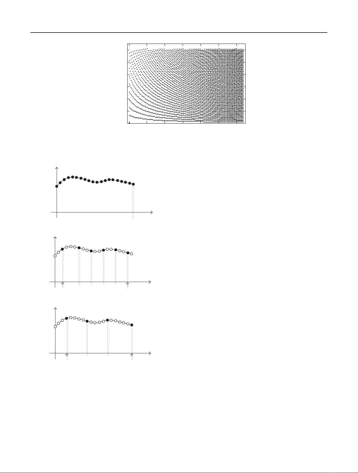
where round(x)convertsxto the nearest integer. Figure 2
contains the plot of index(T,j) as a function of T, with the
position of the index marked by a black dot. As we can see,
vertical separation between dots shrinks as the period in-
creases.
Theschemeworksasfollows:avectoruihaving the same
dimension as xis extracted from the codevector yiby calcu-
lating a set of indices using the associated pitch period. These
indices point to the positions of the codevector where ele-
ments are extracted. The idea is illustrated in Figure 3 and
can be summarized by
ui=C(T)yi(18)
with C(T) the selection matrix associated with the pitch pe-
riod Tand having the dimension N(T)×Nv. The selection
Vector Quantization of Harmonic Magnitudes 2605
20 40 60 80 100 120 140
T
0
20
40
60
80
100
120
Index (T,j)
Figure 2: Indices to the codevectors’ elements as a function of the pitch period T∈[20, 147] when Nv=129.
0Nv−1
y
Index (T1,1) Index(T1,N(T1))
C(T1)y
Index (T2,1) Index(T2,N(T2))
C(T2)y
Figure 3: Illustration of codevector sampling: the original codevec-
tor with Nvelements (top) and two sampling results where T1>T
2.
matrix is specified with
C(T)=c(T)
j,m|j=1,...,N(T); m=0,...,Nv−1,
c(T)
j,m=
1 if index(T,j)=m,
0 otherwise.
(19)
3.2. Codebook generation
We assume that the set of training data
xk,Tk,k=0, ...,Nt−1, (20)
is available, with Ntthe size of the training set. Each vector xk
within the set has a pitch period Tkassociated with it, which
determines the dimension of the vector. The Nccodevectors
divide the whole space into Nccells. The vector xkis said to
pertain to the ith cell if
dCTkyi,xk≤dCTkyj,xk(21)
for all j= i. Thus, given a codebook, we can find the sets
xk,Tk,ik,k=0, ...,Nt−1, (22)
with ik∈[0, Nc−1] the index of the cell that xkpertains to.
The task of obtaining (22)isreferredtoasnearest-neighbor
search [3, page 363]. The objective of codebook generation is
to minimize the sum of distortion at each cell
Di=
k|ik=i
dxk,CTkyi,i=0, ...,Nc−1, (23)
by optimizing the codevector yi;theprocessisreferredtoas
centroid computation. Nearest-neighbor search together with
centroid computation are the key steps of the generalized
Lloyd algorithm (GLA [3, page 363]) and can be used to gen-
erate the codebook. Depending on the selected distance mea-
sure, centroid computation is performed differently. Con-
sider the distance definition
dxk,CTkyi=
xk−CTkyi+gk,i1
2.(24)
Itisassumedin(
24) that all elements of the vectors xkand yi
are in dB values, hence (24) is proportional to SD2as given in
(4). Note that in (24)1is a vector whose elements are all 1’s
with dimension N(T). The variable gk,iis referred to as the
gain and has to be found for each combination of input vec-
tor xk, pitch period Tk,andcodevectoryi. The optimal gain


![PET/CT trong ung thư phổi: Báo cáo [Năm]](https://cdn.tailieu.vn/images/document/thumbnail/2024/20240705/sanhobien01/135x160/8121720150427.jpg)