Independence Complexes of Stable Kneser Graphs
Benjamin Braun∗ Department of Mathematics University of Kentucky, Lexington, KY 40506
benjamin.braun@uky.edu
Submitted: Nov 1, 2010; Accepted: May 10, 2011; Published: May 23, 2011 Mathematics Subject Classification: Primary 05C69, Secondary 57M15
Abstract
For integers n ≥ 1, k ≥ 0, the stable Kneser graph SGn,k (also called the Schrijver graph) has as vertex set the stable n-subsets of [2n + k] and as edges disjoint pairs of n-subsets, where a stable n-subset is one that does not contain any 2-subset of the form {i, i + 1} or {1, 2n + k}. The stable Kneser graphs have been an interesting object of study since the late 1970’s when A. Schrijver determined that they are a vertex critical class of graphs with chromatic number k + 2. This article contains a study of the independence complexes of SGn,k for small values of n and k. Our contributions are two-fold: first, we prove that the homotopy type of the independence complex of SG2,k is a wedge of spheres of dimension two. Second, we determine the homotopy types of the independence complexes of certain graphs related to SGn,2.
1 Introduction
Let [n] := {1, 2, 3, . . . , n} and consider the following family of graphs.
∗The author was partially supported by the NSF through award DMS-0758321. Thanks to the referees for their careful reading of the document. The author is particularly grateful to the anonymous referee who pointed out that Theorem 1.5 can be proved using the contractible subcomplex approach given in the first proof. Thanks also to John Shareshian for thoughtful discussions at the beginning of this project.
the electronic journal of combinatorics 18 (2011), #P118
1
Definition 1.1 For each pair of integers n ≥ 1, k ≥ 0, the Kneser graph KGn,k has as vertices the n-subsets of [2n + k] with edges defined by disjoint pairs of n-subsets. For the same parameters, the stable Kneser graph SGn,k, also called the Schrijver graph, is the subgraph of KGn,k induced by the stable n-subsets of [2n + k], i.e. those n-subsets that do not contain any 2-subset of the form {i, i + 1} or {1, 2n + k}.
The Kneser and stable Kneser graphs have interesting properties related to indepen- dent sets of vertices, where a collection of vertices in a graph G is an independent set if the vertices are pairwise non-adjacent in G. Perhaps the most widely-known structure in graph theory related to independent sets is that of a proper graph coloring, i.e. a partition of the vertices of G into disjoint independent sets. The minimal number of independent sets required for such a partition is called the chromatic number of G and is denoted χ(G). In 1978, L. Lov´asz proved in [13] that χ(KGn,k) = k + 2 by using an ingenious application of the Borsuk-Ulam theorem, thus verifying a conjecture due to M. Kneser from 1955. Shortly afterwards, A. Schrijver determined in [15] that χ(SGn,k) = χ(KGn,k), again us- ing the Borsuk-Ulam theorem. Schrijver also proved that the stable Kneser graphs are vertex critical, i.e. the chromatic number of any subgraph of a stable Kneser graph SGn,k obtained by removing vertices is strictly less than χ(SGn,k). These theorems were one source of inspiration for subsequent work involving the interaction of combinatorics and algebraic topology, see [10, 11, 14] for recent textbook accounts of further developments. Recall that an (abstract) simplicial complex ∆ = (V, F ) is a finite set V , called the vertices of ∆, together with a collection of subsets F ⊆ 2V such that
F ∈ F , G ⊆ F ⇒ G ∈ F ,
called the faces of ∆. For technical purposes, we include the emptyset as a face. Lov´asz’s original proof that χ(KGn,k) = k +2 followed from a general theorem bounding χ(G) from below by a function of the connectivity of the neighborhood complex of G, the complex whose vertices are the vertices of G and whose faces are vertices sharing a common neigh- bor. In [2], Bj¨orner and De Longueville proved that the neighborhood complex of SGn,k is homotopy equivalent to a k-sphere, implying that SGn,k is well-behaved topologically with regard to this construction and Lov´asz’s theorem. While the neighborhood complex plays a fundamental role in providing topological lower bounds on chromatic numbers, this is not the only topological construction that investigates independence structures. If one is interested in the interplay among all the independent sets in G, without regard to chromatic numbers, one is led to the following construction.
Definition 1.2 Let G = (V, E) be a graph. The independence complex of G, Ind(G), is the simplicial complex with vertex set V and faces given by independent sets.
Independence complexes have been the subject of recent investigation, see for exam- ple [3, 5, 6, 7, 9, 17]. Five of these papers involve a connection between independence complexes of graphs and hard squares models in statistical mechanics. Additionally, the homotopy type of the independence complexes of cycles played a critical role in the recent resolution by E. Babson and D. Kozlov in [1] of Lov´asz’s conjecture regarding odd cycles and graph homomorphism complexes.
the electronic journal of combinatorics 18 (2011), #P118
2
Our purpose in this paper is to investigate the homotopy type of the independence complexes of the stable Kneser graphs SG2,k and the independence complexes of a family of graphs related to SGn,2. There are several reasons to be curious about the indepen- dence complex of SGn,k. Since the stable Kneser graphs are vertex-critical, they are a
minimal obstruction to colorability in the Kneser graphs, and the chromatic number in- herently measures some restricted behavior of independent sets which is reflected in the neighborhood complex. It is of interest to see what, if any, properties of independent sets in SGn,k are exposed through Ind(SGn,k). Also, an independent set in SGn,k is a pairwise intersecting family of stable n-subsets of [2n + k]. Such families have been previously studied from an extremal perspective, see for example [16] and the references therein.
The homotopy types of the independence complexes of some stable Kneser graphs are already known. For n = 1, the stable Kneser graphs are complete graphs and thus their independence complexes are wedges of 0-dimensional spheres. For k = 0, the stable Kneser graphs are complete graphs on two vertices, hence their independence complexes are zero dimensional spheres. For k = 1, it is easy to see that SGn,1 = C2n+1, the cycle of odd length, and the homotopy types of independence complexes of cycles are known.
Theorem 1.3 (Kozlov, [12]) For n ≥ 1, let Cn denote the cycle of length n. The following homotopy equivalence holds:
Sr−1 Ind(Cn) ≃ Sr−1 Sr−1 if n = 3r if n = 3r ± 1 (cid:26) W
Our first contribution is to describe Ind(SG2,k) up to homotopy.
Theorem 1.4 For k ≥ 4,
−1
6
S2. Ind(SG2,k) ≃ _(k−3)(k−1)(k+4)
Also,
S1 Ind(SG2,2) ≃ S1 _ and
Ind(SG2,3) ≃ S1.
Our second contribution is to investigate Ind(SGn,2). Unfortunately, as will be dis- cussed in Section 4, these complexes are more complicated than those where n = 2, and their homotopy type is still unknown. However, we will be able to determine the homo- topy type of a class of graphs we call E2n+2, close relatives of SGn,2 that will be defined in Section 4. A rough description of SGn,2 is as a cylinder graph with some additional edges on the cycles forming the ends of the cylinder; E2n+2 is then obtained by “squeezing” SGn,2 so that only the end cycles and additional edges remain.
Theorem 1.5 Let n ≥ 3. If 4 | 2n + 2, i.e. n is odd, then
the electronic journal of combinatorics 18 (2011), #P118
3
S2k+1 S2k+1 . Ind(E2n+2) ≃ S2k+1 S2k+2 if n = 4k + 1 if n = 4k + 3 (cid:26) W W
If 4 ∤ 2n + 2, i.e. n is even, then
S2k+1 . Ind(E2n+2) ≃ S2k S2k+1 S2k+2 if n = 6k if n = 6k + 2 if n = 6k + 4 W
In Section 3, we prove Theorem 1.4.
Our primary tool for proving these theorems is discrete Morse theory. The remainder In Section 2, we discuss the basics of discrete of the paper is structured as follows. Morse theory, including the construction of acyclic partial matchings via matching trees introduced in [3]. In Section 4, we provide an explicit description of the graphs SGn,2 leading to the definition of E2n+2 and remark on a connection between Ind(SGn,2) and [9]. Finally, in Section 5 we provide a proof of Theorem 1.5.
2 Tools From Discrete Morse Theory
In this section we introduce the tools we need from discrete Morse theory. Discrete Morse theory was introduced by R. Forman in [8] and has since become a standard tool in topological combinatorics. The main idea of (simplicial) discrete Morse theory is to pair cells in a simplicial complex in a manner that allows them to be cancelled via elementary collapses, reducing the complex under consideration to a homotopy equivalent complex, cellular but possibly non-simplicial, with fewer cells. Detailed discussions of the following definitions and theorems, along with their proofs, can be found in [10, 11].
2.1 Partial Matchings and the Main Theorem
Definition 2.1 A partial matching in a poset P is a partial matching in the underlying graph of the Hasse diagram of P , i.e. it is a subset M ⊆ P × P such that
• (a, b) ∈ M implies b covers a, i.e. a < b and no c satisfies a < c < b, and
• each a ∈ P belongs to at most one element in M.
When (a, b) ∈ M we write a = d(b) and b = u(a). A partial matching on P is called acyclic if there does not exist a cycle
b1 > d(b1) < b2 > d(b2) < · · · < bn > d(bn) < b1,
with n ≥ 2, and all bi ∈ P being distinct.
the electronic journal of combinatorics 18 (2011), #P118
4
Given an acyclic partial matching M on P , we say that the unmatched elements of P are critical. The following theorem asserts that an acyclic partial matching on the face poset of a polyhedral cell complex is exactly the pairing needed to produce our desired homotopy equivalence.
Theorem 2.2 (Main Theorem of Discrete Morse Theory) Let ∆ be a polyhedral cell com- plex and let M be an acyclic partial matching on the face poset of ∆. Let ci denote the number of critical i-dimensional cells of ∆. The space ∆ is homotopy equivalent to a cell complex ∆c with ci cells of dimension i for each i ≥ 0, plus a single 0-dimensional cell in the case where the emptyset is paired in the matching.
Remark 2.3 In particular, if an acyclic partial matching M has critical cells only in a fixed dimension i, then ∆ is homotopy equivalent to a wedge of i-dimensional spheres.
It is often useful to be able to make acyclic partial matchings on different sections of a poset and combine them to form a larger acyclic partial matching. This process is formalized via the following theorem, referred to as the Cluster Lemma in [10, Lemma 4.2] and the Patchwork Theorem in [11, Theorem 11.10].
Theorem 2.4 If φ : P → Q is an order-preserving map and, for each q ∈ Q, each subposet φ−1(q) carries an acyclic partial matching Mq, then the union of the Mq is an acyclic partial matching on P .
2.2 Matching Trees
To facilitate the study of Ind(G) for a graph G = (V, E), matching trees were introduced by Bousquet-M´elou, et al. in [3, Section 2]. Let
a∈A N(a) ⊆ B, where N(a) denotes
Σ(A, B) := {I ∈ Ind(G) : A ⊆ I and B ∩ I = ∅} ,
where A, B ⊆ V satisfy A ∩ B = ∅ and N(A) := the neighbors of a in G. S
Definition 2.5 Let G be a connected graph. A matching tree, M(G), for G is a directed tree constructed according to the following algorithm. Begin by letting M(G) be a single node labeled Σ(∅, ∅), and consider this node a sink until after the first iteration of the following loop:
WHILE M(G) has a leaf node Σ(A, B) that is a sink with |Σ(A, B)| ≥ 2 DO ONE OF THE FOLLOWING
1. If there exists a vertex p ∈ V \ (A ∪ B) such that
|N(p) \ (A ∪ B)| = 0,
the electronic journal of combinatorics 18 (2011), #P118
5
create a directed edge from Σ(A, B) to a new node labeled ∅. Refer to p as a free vertex of M(G).
2. If there exist vertices p ∈ V \ (A ∪ B) and v ∈ N(p) such that
N(p) \ (A ∪ B) = {v},
create a directed edge from Σ(A, B) to a new node labeled
Σ(A ∪ {v}, B ∪ N(v)).
Refer to v as a matching vertex of M(G) with respect to p.
3. Choose a vertex v ∈ V \ (A ∪ B) and created two directed edges from Σ(A, B) to new nodes labeled Σ(A, B ∪ {v})
and Σ(A ∪ {v}, B ∪ N(v)).
Refer to v as a splitting vertex of M(G).
The node Σ(∅, ∅) is called the root of the matching tree, while any non-root node of degree 2 in M(G) is called a matching site of M(G) and any non-root node of degree 3 is called a splitting site of M(G).
The key observation in [3] is that a matching tree on G yields an acyclic partial matching on the face poset of Ind(G), as the following theorem indicates.
Theorem 2.6 [3, Section 2] A matching tree M(G) for G yields an acyclic partial match- ing on the face poset of Ind(G) whose critical cells are given by the non-empty sets Σ(A, B) labeling non-root leaves of M(G). In particular, for such a set Σ(A, B), the set A yields a critical cell in Ind(G).
3 Proof of Theorem 1.4
The case k = 2 is a simple exercise, as the complex is pure two-dimensional and has only eight maximal faces. The case k = 3 is handled at the end of this section. Let k ≥ 4 and let Qk denote the face poset of Ind(SG2,k) and let Ik+2 be a (k + 2)-element chain, with elements labeled 3 < 4 < 5 < 6 < · · · < k + 4. Our goal is to create an acyclic partial matching on Qk by using Theorem 2.4 to break Qk into preimages and produce acyclic partial matchings on these. In this section, addition and subtraction are modulo k + 4. Note that in our proof below, whenever a 2-element subset {i, j} is considered, it is assumed that {i, j} is stable, i.e. |i − j| ≥ 2 and {i, j} 6= {1, k + 4}.
the electronic journal of combinatorics 18 (2011), #P118
6
While the maps and matchings below appear complicated, they are easily motivated. The maximal elements of Qk are of two types: independent sets of the form {{i, j} : j ∈ [k +4]}, and independent sets of the form Ti,j,h := {{{i, j}, {j, h}, {i, h}} : i, j, h ∈ [k +4]}. Thus, Ind(SG2,k) is built from k + 4 simplices of dimension k and additional 2-cells. Our
goal is to cut down the k-dimensional facets so that only faces of small dimension remain. Informally, we want to begin this process by pairing faces σ with σ ∪ {1, 3} when possible, which leads us to begin defining a map φ : Qk → Ik+2 as follows. Note that all variables referenced (e.g. j, r, i1, i2, . . .) are integers in [k + 4].
σ ⊆ {{1, j} : j ∈ [k + 4]} σ ⊆ {{3, j} : j ∈ [k + 4]} φ−1(3) :=
∅ σ σ {{1, j}, {3, j}} 3 < j < k + 4 3 < j < k + 4 T1,3,j
To continue our definition of φ, we remark that from the remaining unpaired faces, we eventually want to pair σ with σ ∪ {1, 4} when possible; once this is done, we will want to pair σ with σ ∪ {1, 5} when possible, etc. Continuing this process until reaching k + 3 leads us to continue defining the map φ as follows. For 3 < l < k + 4,
φ−1(l) :=
{2, l} {{1, l}, {2, l}} {l, j} l < j ≤ k + 4 {{l, i}, {l, j}} l < i < j ≤ k + 4 {{i, l}, {l, j}} 1 ≤ i < l < j ≤ k + 4 2 ≤ i < j < l {{i, l}, {j, l}} {{l, i1}, {l, i2}, . . . , {l, ir}} 3 ≤ r ≤ k + 1 l < j ≤ k + 3 {{1, j}, {l, j}} l < j ≤ k + 3 T1,l,j
To motivate the conclusion of our definition of φ, we remark that following the pairing process, we will be left with additional unpaired faces that are not 2-dimensional. To com- plete our matching, we will construct a second poset map ψ on the remaining “unpaired” elements, so we assign these remaining elements to the preimage φ−1(k + 4):
φ−1(k + 4) :=
i, j, h 6= 1 {2, k + 4} {{2, i1}, {2, i2}, . . . , {2, ir}} 2 ≤ r ≤ k + 1 {{k + 4, i1}, {k + 4, i2}, . . . , {k + 4, ir}} 2 ≤ r ≤ k + 1 Ti,j,h
It is straightforward to check that φ is an order-preserving map. For 3 ≤ l < k + 4, we produce an acyclic matching Ml on φ−1(l) via the matching (σ, σ ∪ {1, l}) for each σ not containing {1, l}. It is straightforward to check that for each l, every element of φ−1(l) is an element of some matched pair in Ml. Ml is acyclic because if one attempts to construct a directed cycle in φ−1(l) as in Definition 2.1, starting from an element σ not containing {1, l}, we must begin our cycle with
the electronic journal of combinatorics 18 (2011), #P118
7
σ < σ ∪ {1, l} < (σ ∪ {1, l}) \ {i, j}
for some {i, j} 6= {1, l}. However, there is no τ ∈ Qk such that σ′ := (σ ∪ {1, l}) \ {i, j} satisfies (σ′, τ ) ∈ Ml, hence we cannot complete our desired cycle.
Remaining is only the poset φ−1(k + 4). To establish an acyclic partial matching here, we apply Theorem 2.4 a second time. Observe that the elements of φ−1(k + 4) are parts of “stars” through 2 or k + 4, together with triangles that avoid 1. Let C := {b < r6 < r7 < · · · < rk+3 < m1 < m2 < t2 < s4 < s5 < · · · < sk+2 < m3 < m4 < tk+4} be a chain; we will define our map ψ : φ−1(k + 4) → C in two steps. First, we define preimages under ψ that will host pairings eliminating unwanted faces containing 2.
ψ−1(b) := {2, k + 4} {{2, 4}, {2, k + 4}} (cid:26)
For 6 ≤ i ≤ k + 3,
ψ−1(ri) := {{2, 4}, {2, i}} {{2, 4}, {2, i}, {4, i}} (cid:26)
ψ−1(m1) := {{2, 5}, {2, 7}} {{2, 5}, {2, 7}, {5, 7}} (cid:26)
ψ−1(m2) := {{2, 4}, {2, 5}} {{2, 4}, {2, 5}, {2, 7}} (cid:26)
5 ≤ i < j ≤ k + 4
ψ−1(t2) := 3 ≤ r ≤ k + 1 {{2, i}, {2, j}} except {{2, 5}, {2, 7}} {{2, i1}, {2, i2}, . . . , {2, ir}} except {{2, 4}, {2, 5}, {2, 7}}
Observe that most of these preimages contain exactly an edge and a triangle that we will end up pairing together, and in the preimage ψ−1(t2) is found the remaining faces coming from the “star” through 2. Next, we need to define preimages under ψ that will host pairings eliminating unwanted faces containing k + 4. For 4 ≤ j ≤ k + 2,
ψ−1(sj) := {{2, k + 4}, {j, k + 4}} {{2, k + 4}, {j, k + 4}, {2, j}} (cid:26)
ψ−1(m3) := {{3, k + 4}, {5, k + 4}} {{3, k + 4}, {5, k + 4}, {3, 5}} (cid:26)
ψ−1(m4) := {{2, k + 4}, {3, k + 4}} {{2, k + 4}, {3, k + 4}, {5, k + 4}} (cid:26)
3 ≤ i < j < k + 4
3 ≤ r ≤ k + 1 ψ−1(tk+4) :=
{{i, k + 4}, {j, k + 4}} except {{3, k + 4}, {5, k + 4}} {{k + 4, i1}, {k + 4, i2}, . . . , {k + 4, ir}} except {{2, k + 4}, {3, k + 4}, {5, k + 4}} Ti,j,k Ti,j,k not yet listed
the electronic journal of combinatorics 18 (2011), #P118
8
Observe again that most of these preimages contain exactly an edge and a triangle that we will end up pairing together, and in the preimage ψ−1(tk+4) is found the remaining faces coming from the “star” through k + 4.
It is straightforward to check that this is an order preserving map. To form acyclic partial matchings on these preimages, for all elements in the chain except t2 and tk+4, match the pair of elements in the preimage. Match the pair (σ, σ ∪ {2, 4}) on ψ−1(t2); this matching is acyclic and matches every element. Match the pair (σ, σ ∪ {2, k + 4}) on ψ−1(tk+4); this matching is again acyclic, but does not match every element. One can check that the critical cells on ψ−1(tk+4) are given by the set
Mcrit := {Ti,j,h : i < j < h, i, j, h 6= 1} \ S,
where
k+1 3
S := {T2,4,j : 6 ≤ j ≤ k + 3} ∪ {T2,j,k+4 : 4 ≤ j ≤ k + 2} ∪ {T3,5,k+4, T2,5,7}.
It is straightforward to calculate that the size of {Ti,j,h : i < j < h, i, j, h 6= 1} is and the size of S is 2k − 1, hence the size of Mcrit is (cid:0) (cid:1)
k + 1 − (2k − 1) = − 1, (k − 3)(k − 1)(k + 4) 6 (cid:18) 3 (cid:19)
as desired. We are now in a position to invoke Theorems 2.2 and 2.4, completing our proof for the case k ≥ 4.
For the case k = 3, we define φ as above, but we must modify the definition of ψ. In particular, for this case we eliminate ψ−1(m1) and ψ−1(m2) and include {{2, 5}, {2, 7}}, {{2, 4}, {2, 5}} and {{2, 4}, {2, 5}, {2, 7}} in ψ−1(t2). Note that the triangle T2,5,7 is already present in ψ−1(s5). There are only four stable triangles avoiding 1, namely T2,4,6, T2,4,7, T2,5,7 and T3,5,7. These four cells are paired individually in the preimages of r6, s4, s5, and m3, respectively, implying that there are no unlisted triangles contained in ψ−1(t7). Thus, for the case k = 3, the only critical cell is {{2, 4}, {2, 5}}, and our proof is complete.
4 The graphs SGn,2 and E2n+2
The graphs SGn,2 admit an alternate description which we will discuss here. This de- scription is given in detail in [4], but the details are easy to fill in from the following. For an integer n ≥ 2, we define:
if 2 ∤ n p(n) := n n − 1 otherwise (cid:26)
n+1 2 n+2 2
the electronic journal of combinatorics 18 (2011), #P118
9
o(n) := if 2 | n + 1 otherwise (cid:26)
Observe that a vertex of SGn,2 is given by a stable n-subset of [2n + 2] and that these subsets may be partitioned into three classes.
Definition 4.1 Let X := {i1, i2, . . . , in} be a stable n-subset of [2n + 2], where [2n + 2] is ordered cyclically.
A: We say X is an alternating end vertex if X is an image
α({1, 3, . . . , p(n), p(n) + 3, p(n) + 5, . . . , 2n})
for some permutation α of the stable n-subsets of [2n + 2] induced by a cyclic per- mutation of [2n + 2];
B: We say X is a bipartite end vertex if X is a proper subset of either the even numbers or the odd numbers; and
{2,4,6,9}
(cid:0)(cid:1) (cid:0)(cid:1)
{1,3,5,7}
(cid:0)(cid:1)
(cid:0)(cid:1)(cid:0)(cid:0)(cid:1)(cid:1)
(cid:1)(cid:1) (cid:0)(cid:0) (cid:0)(cid:0) (cid:1)(cid:1)
{1,4,6,9}
(cid:0)(cid:1)
(cid:1)(cid:1) (cid:0)(cid:0) (cid:0)(cid:0) (cid:1)(cid:1)
(cid:0)(cid:0)(cid:1)(cid:1)
{2,4,6,8}
(cid:0)(cid:0)(cid:1)(cid:1) (cid:0)(cid:1)
(cid:0)(cid:1)
(cid:1)(cid:1) (cid:0)(cid:0) (cid:0)(cid:0) (cid:1)(cid:1)
{3,5,7,10}
(cid:0)(cid:1)
(cid:1) (cid:0) (cid:1)(cid:1)(cid:1)(cid:1)(cid:1) (cid:0)(cid:0)(cid:0)(cid:0)(cid:0) (cid:0) (cid:1) (cid:0)(cid:0)(cid:0)(cid:0)(cid:0) (cid:1)(cid:1)(cid:1)(cid:1)(cid:1) (cid:0)(cid:0)(cid:0)(cid:0)(cid:0) (cid:1)(cid:1)(cid:1)(cid:1)(cid:1) (cid:1)(cid:1) (cid:0)(cid:0) (cid:0)(cid:0)(cid:0)(cid:0)(cid:0) (cid:1)(cid:1)(cid:1)(cid:1)(cid:1) (cid:0)(cid:0) (cid:1)(cid:1) (cid:1) (cid:0) (cid:0)(cid:0)(cid:1)(cid:1) (cid:0)(cid:0)(cid:0)(cid:0)(cid:0) (cid:1)(cid:1)(cid:1)(cid:1)(cid:1) (cid:1) (cid:0) (cid:0)(cid:0)(cid:0)(cid:0)(cid:0) (cid:1)(cid:1)(cid:1)(cid:1)(cid:1) (cid:0)(cid:1)
{3,5,7,9}
(cid:0)(cid:0)(cid:1)(cid:1)
(cid:0)(cid:0)(cid:1)(cid:1)(cid:0)(cid:1)
(cid:0)(cid:1)
(cid:0)(cid:0)(cid:1)(cid:1)
(cid:0)(cid:1)
{4,6,8,10}
M: We say X is a middle vertex for all other cases.
Figure 1: SG4,2
the electronic journal of combinatorics 18 (2011), #P118
10
Figures 1 and 2 contain representations of SG4,2 and SG5,2 which we will use as references throughout this discussion. Recall that given two graphs G and H, the cartesian product G(cid:3)H has vertex set V (G) × V (H) with (u, v) adjacent to (u′, v′) if and only if u = u′ and {v, v′} ∈ E(H), or v = v′ and {u, u′} ∈ E(G). Note that each copy of SGn,2 contains a complete bipartite graph Kn+1,n+1 induced by the bipartite end vertices of SGn,2, hence the nomenclature. In Figures 1 and 2, these vertices are the outer ring of the graph, where for visual clarity we have not displayed all the edges, replacing them instead with dashed lines at each vertex indicating the presence of an edge. Let Cj denote the cycle of length j and let Pj denote the path with j vertices. For every n, the middle vertices of SGn,2 induce as a subgraph a copy of C2n+2(cid:3)Po(n)−2 which we call the middle cylinder. In our examples above, o(4) = o(5) = 3, and hence the middle rings of vertices in Figures 1 and 2 are C10(cid:3)P1 and C12(cid:3)P1, respectively. It is easy to see that each bipartite end vertex of SGn,2 is connected to a unique vertex on an end cycle of the
{2,4,6,8,12}
(cid:1) (cid:0) (cid:0)(cid:1) (cid:0) (cid:1)
(cid:0)(cid:0)(cid:1)(cid:1)
(cid:0)(cid:0)(cid:1)(cid:1)
{2,4,6,8,11}
(cid:1)(cid:1) (cid:0)(cid:0) (cid:0) (cid:1)(cid:0)(cid:0) (cid:1)(cid:1) (cid:0) (cid:1)
{1,3,5,7,9}
(cid:0)(cid:1)(cid:0)(cid:0)(cid:1)(cid:1) (cid:0)(cid:1)
(cid:0)(cid:1)
(cid:1)(cid:1) (cid:0)(cid:0) (cid:0)(cid:0) (cid:1)(cid:1)
{3,5,7,10,12}
(cid:0)(cid:0)(cid:1)(cid:1)
(cid:0)(cid:0)(cid:1)(cid:1)
(cid:1) (cid:0) (cid:0) (cid:1)
{2,4,6,8,10}
(cid:0)(cid:1)
(cid:0)(cid:1)
(cid:0)(cid:1) (cid:1)(cid:1) (cid:0)(cid:0) (cid:0)(cid:0) (cid:1)(cid:1) (cid:1)(cid:1) (cid:0)(cid:0) (cid:0)(cid:1) (cid:0)(cid:0) (cid:1)(cid:1) (cid:0)(cid:1) (cid:0)(cid:1) (cid:1) (cid:0) (cid:0)(cid:0)(cid:1)(cid:1) (cid:1) (cid:0) (cid:1) (cid:0) (cid:0)(cid:0) (cid:1)(cid:1) (cid:1) (cid:0) (cid:0)(cid:0) (cid:1)(cid:1)
(cid:1) (cid:0) (cid:0) (cid:1) (cid:0)(cid:0)(cid:1)(cid:1) (cid:0)(cid:0)(cid:1)(cid:1) (cid:1) (cid:0) (cid:0) (cid:1)
{3,5,7,9,12}
(cid:0)(cid:1)(cid:0)(cid:1)
(cid:0)(cid:1)
(cid:0)(cid:0)(cid:1)(cid:1)
(cid:0)(cid:1)
(cid:1) (cid:0) (cid:0) (cid:1)
{3,5,7,9,11}
Figure 2: SG5,2
middle cylinder. Finally, the alternating end vertices of SGn,2 induce a copy of Cn+1 in the case when 2 | n and a copy of DC2n+2 in the case when 2 ∤ n, where DC2n+2 is defined to be a (2n + 2)-cycle augmented by edges connecting antipodal vertices. In the first case, each alternating end vertex of SGn,2 is connected to a pair of middle vertices, while in the latter case each alternating end vertex of SGn,2 is connected to a unique middle vertex. A moment of thought reveals that when n is even, there are n + 1 alternating end vertices, while for n odd there are 2n + 2 alternating end vertices, and there are 2n + 2 bipartite end vertices and (2n + 2) · (o(n) − 2) middle vertices.
Remark 4.2 In the case where n is odd, the graph SGn,2 can be described as an even cylinder C2n+2(cid:3)Po(n) with additional edges forming a complete bipartite graph on one end and a cycle with diagonals on the other end, with a similar description for n even. Though the graphs SGn,2 admit this nice description, the complexes Ind(SGn,2) have been resistant to investigation. The difficult nature of this problem is similar to the difficult nature of the study of Ind(C2n+2(cid:3)Pl) for arbitrary l ≥ 6, n ≥ 3. As discussed in Section 6 of [9], even a determination of the Euler characteristic of Ind(C2n+2(cid:3)Pl) is unknown in general. For small values of n and l, there are some results regarding the homotopy type and Euler characteristic of these complexes, e.g. [17], but in general this is an interesting open problem.
the electronic journal of combinatorics 18 (2011), #P118
11
One approach for studying Ind(SGn,2) would be to consider arbitrary even circumfer- ence cylinders C2n+2(cid:3)Pl and augment their end cycles in a manner consistent with that described above. One might hope to then induct on l in some fashion, though our at- tempts following this approach have been unsuccessful. However, were one to pursue this strategy, the base case would be a cylinder of length two, i.e. a cylinder with no middle vertices. We therefore introduce the following class of graphs, which are formed by consid- ering only the end vertices of SGn,2 and connecting them directly via edges. Let Kn+1,n+1 denote the complete bipartite graph on vertex set {1, 2, . . . , 2n + 2} with bipartition into the set of odds and evens. Let DC2n+2 denote the cycle on the vertex set {c1, c2, . . . , c2n+2} with edges {{ci, ci+1} : i ∈ [2n+2]}∪{{ci, ci+n+1} : i ∈ [n+1]}. Let Cn+1 denote the cycle
on the vertex set {c1, c3, c5, . . . , c2n+1} with edges {{ci, ci+2} : i ∈ {1, 3, 5, . . . , 2n + 1}}. For all of these graphs, addition of indices for vertices is modulo 2n + 2.
Definition 4.3 For n ≥ 2, let E2n+2 denote the following graph: if 2 ∤ n, take a copy of Kn+1,n+1 and a copy of DC2n+2 and add an edge connecting each vertex i of Kn+1,n+1 to the vertex ci of DC2n+2. If 2 | n, take a copy of Kn+1,n+1 and a copy of Cn+1 and add edges connecting each vertex ci of Cn+1 to the vertices i and i + n + 1 of Kn+1,n+1.
Remark 4.4 As Theorem 1.5 indicates, the topology of Ind(E2n+2) is reasonably well- behaved. It would be of interest to understand more about the topology of the independence complexes of the graphs obtained by adding middle cycles back into E2n+2; in particular, it would be interesting to know if there is any relation between the independence complexes of the graphs obtained by adding j middle cycles and j + k middle cycles to E2n+2 for small values of k.
5 Proof of Theorem 1.5
We will sketch two proofs of Theorem 1.5. The idea behind the first proof is that Ind(E2n+2) can be covered by two contractible subcomplexes that intersect in the in- dependence complex of Cn+1 or DC2n+2, depending on the parity of n. Thus, Ind(E2n+2) is the suspension of the independence complex of the relevant graph. For the second proof, we will show how to construct matching trees for the some of the graphs E2n+2. While the second proof is significantly longer than the first, we provide this sketch because matching trees are one approach to the questions discussed in Remark 4.4. The author cannot see how the techniques used in the first proof might easily extend to the general case.
When we use matching trees in the following, we refer to vertices of the matching tree as nodes, reserving the word vertices for the vertices of E2n+2. During the construction of our trees, references to matching, splitting, and free vertices of E2n+2 are references to the types of vertices possible in the matching tree construction algorithm given in Section 2. It is helpful to use diagrams like Figure 4 to illustrate matching trees, which we also describe with Σ(A, B) notation. In these diagrams, each node of the matching tree is shown as a graph representing Σ(A, B), where black dots represent elements of A, white dots represent elements of B, and gray dots represent elements in neither A nor B. Both proofs below involve the following definition and lemma.
Definition 5.1 Let EL0 := K2 and let EL1 := K1,3, where K1,3 is a complete bipartite graph with bipartition sets of size 1 and 3. For r ≥ 2, let ELr be the graph with 2r + 2 vertices depicted in Figure 3.
Lemma 5.2 There is a matching tree on ELr with a single non-empty leaf corresponding to a critical cell of size
, 2k + 1 2k + 1 if r = 4k if r = 4k + 1 (cid:26)
the electronic journal of combinatorics 18 (2011), #P118
12
and no critical cell if r = 4k + 2 or r = 4k + 3.
(cid:0)(cid:1) (cid:0)(cid:1)
(cid:0)(cid:1)(cid:0)(cid:0)(cid:1)(cid:1)
(cid:0)(cid:1)
(cid:0)(cid:1)
(cid:0)(cid:1) (cid:0)(cid:1)
(cid:1) (cid:0) (cid:0) (cid:1)
(cid:1) (cid:0) (cid:0) (cid:1)
(cid:1) (cid:0) (cid:0) (cid:1)
(cid:1)(cid:1) (cid:0)(cid:0) (cid:0)(cid:0) (cid:1)(cid:1)
(cid:1) (cid:0) (cid:0) (cid:1)
(cid:1) (cid:0) (cid:0) (cid:1)
(cid:1) (cid:0) (cid:0) (cid:1)
(cid:1) (cid:0) (cid:0) (cid:1)
(cid:1)(cid:1) (cid:0)(cid:0) (cid:0)(cid:0) (cid:1)(cid:1)
(cid:1) (cid:0) (cid:0) (cid:1) a
b
Figure 3:
Proof: It is straightforward to construct a matching tree taking ELr to ELr−4 by first using the vertex labeled a as a matching vertex, then using b as a matching vertex. Iterate this process until the only gray vertices remaining form a copy of ELr for r = 0, 1, 2, or 3. At each iteration, exactly two black vertices are added. It is now an easy exercise to check that there are matching trees on EL0 and EL1 yielding a single non-empty leaf with a single black vertex, while there are matching trees on EL2 and EL3 with no critical cells. (cid:3)
5.1 Proof by covering with contractible subcomplexes
We apply the gluing lemma, Theorem 15.25 in [11], which implies that if a complex X is covered by two contractible subcomplexes A and B, then X is homotopy equivalent to the suspension of A ∩ B. We will cover Ind(E2n+2) by the subcomplexes arising as independence complexes of the subgraphs of E2n+2 induced by DC2n+2, when n is odd, or Cn+1, when n is even, together with the n + 1 vertices from a shore of Kn+1,n+1.
That these subcomplexes are contractible follows from Lemma 2.4 of [6], stating that for any graph G and two vertices v, w in G, if the neighborhood of v is contained in the neighborhood of w, then Ind(G) is homotopy equivalent to Ind(G − {w}). Specifically, when n is even, this lemma allows us to eliminate every vertex in Cn+1 from our subcom- plexes, with only a simplex remaining. When n is odd, this lemma allows us to eliminate every other vertex in DC2n+2 from our subcomplex, and what is left is a join of (n + 1)/2 copies of S0 with a simplex formed by the relevant shore of Kn+1,n+1. In both cases, the two subcomplexes clearly intersect in Ind(DC2n+2) or Ind(Cn+1), and hence the complexes Ind(E2n+2) are suspensions of these. The homotopy type of the independence complex of Cn+1 is given in Theorem 1.3. For DC2n+2, we have the following, which finishes our proof.
Lemma 5.3
S2k S2k . Ind(DC2n+2) ≃ if n = 4k + 1 if n = 4k + 3 (cid:26) S2k S2k+1 W W
the electronic journal of combinatorics 18 (2011), #P118
13
Proof: Construct a matching tree as follows, using the notation introduced just before Definition 4.3. Use c1 as a splitting vertex. On Σ({c1}, {c2, c2n+2, cn+2}), we use cn as a matching vertex and what remains is a copy of ELn−4, plus the two included elements c1 and cn. On Σ(∅, {c1}), we use c2 as a splitting vertex. The case Σ({c2}, {c1, c3, cn+3})
is identical to our first case, yielding a copy of ELn−4 plus the two included elements c2 and cn+1. We are thus left with Σ(∅, {c1, c2}). In this case, it is straightforward to use cn−1 as a splitting vertex and (after a few more obvious steps) have two more nonempty leaves on the tree: a copy of ELn−3 plus one point, and a copy of ELn−5 plus two points. Applying Lemma 5.2 to complete this matching tree finishes the proof. (cid:3)
5.2 Proof by matching tree construction for odd n
The matching tree proof also requires two cases, 4 | 2n + 2 and 4 ∤ 2n + 2; however, as this section is primarily intended to illustrate the matching tree method in this context, we discuss only the first case.
When 4 | 2n + 2, the first step of our matching tree construction proceeds as follows: from Σ(∅, ∅), use vertex 1 as a splitting vertex, yielding directed edges to new nodes Σ({1}, {2, 4, . . . , 2n + 2, c1}) and Σ(∅, {1}). For node Σ({1}, {2, 4, . . . , 2n + 2, c1}), we have that vertex c3 is a matching vertex with respect to vertex 3, thus we can create a directed edge to a new node labeled Σ({1, c3}, {2, 3, 4, 6, . . . , 2n + 2, c2, c4, c3+n+1}). For this node, vertex n + 4 is a free vertex, and we can create a new directed edge to a node labeled ∅. Our construction now proceeds by iterating this first branching step on the node Σ(∅, {1, 2, 3, . . . , i}), where 1 ≤ i ≤ n − 2. After repeating this for all 1 ≤ i ≤ n − 2, our only remaining leaf node in M(E2n+2) is Σ(∅, {1, 2, 3, . . . , n − 1}).
We now proceed by iterating a different matching process where we assume that 0 ≤ r ≤ n − 2 and that M(E2n+2) has only one leaf node, labeled Σ(∅, {1, 2, 3, . . . , n − 1 + r}). We use vertex n + r as a splitting vertex, creating two new edges to nodes labeled
Σ(∅, {1, 2, 3, . . . , n + r})
and
Σ ({n + r}, {1, 2, 3, . . . , n − 1 + r, n + r + 1, n + r + 3, . . . , j, cn+r}) ,
where j is either 2n + 1 or 2n + 2 depending on the parity of n + r. The first node is handled when we consider the case r + 1, while for the second node we use cn+r+2 as a matching vertex with respect to vertex n + r + 2, then use cn+r+4 as a matching vertex with respect to the vertex n + r + 4 to obtain a new edge to a node for which vertex cr+2 is a free vertex, leading us to ∅. Following these iterations, our matching tree has only one non-empty leaf node, labeled Σ(∅, {1, 2, 3, . . . , 2n − 2}), represented as the graph in Figure 4. We next use vertex 2n as a splitting vertex, yielding two new edges to new nodes which we handle in subcases below.
Subcase: Σ({2n}, {1, 2, 3, . . . , 2n − 1, 2n + 1, c2n}) Using vertex c2n+2 as a splitting vertex makes vertex 2n + 2 a free vertex for
Σ({2n}, {1, 2, 3, . . . , 2n − 1, 2n + 1, c2n, c2n+2}),
leaving us to consider only the node
the electronic journal of combinatorics 18 (2011), #P118
14
Σ({2n, c2n+2}, {1, 2, 3, . . . , 2n − 1, 2n + 1, 2n + 2, c2n, c2n+1, c1, cn+1}).
2
1
2n+2
2n+1
2n
2n−2
2n−1
c2n+2
Figure 4: We have suppressed some of the edges in the bipartite graph portion of E2n+2 for clarity.
Using vertex cn−1 as a splitting vertex, we see that vertex cn is a free vertex for
Σ({2n, c2n+2}, {1, 2, 3, . . . , 2n − 1, 2n + 1, 2n + 2, c2n, c2n+1, c1, cn+1, cn−1}),
leaving us to consider only the node
Σ({2n, c2n+2, cn−1}, {1, 2, 3, . . . , 2n − 1, 2n + 1, 2n + 2, c2n, c2n+1, c1, cn+1, cn, cn−2}).
The remaining vertices induce as a subgraph of E2n+2 a copy of ELn−4. Thus, we are in a position to invoke Lemma 5.2, and we see that the portion of the resulting matching tree M(E2n+2) rooted from our remaining node yields a critical cell of size 2k + 2 if n = 4k + 1 and no critical cells if n = 4k + 3.
Subcase: Σ(∅, {1, 2, 3, . . . , 2n − 2, 2n}) Using vertex c2n+2 as a splitting vertex makes vertex 2n + 1 a free vertex for
Σ({c2n+2}, {1, 2, 3, . . . , 2n − 2, 2n, 2n + 2, c1, c2n+1, cn+1}),
leaving us to consider only the node
Σ(∅, {1, 2, 3, . . . , 2n − 2, 2n, c2n+2}).
We now use vertex 2n+1 as a splitting vertex, yielding two new edges to new nodes which we consider in two subsubcases.
Subsubcase: Σ(∅, {1, 2, 3, . . . , 2n − 2, 2n, c2n+2, 2n + 1}) We first use vertex 2n − 1 as a matching vertex with respect to vertex 2n + 2. Using vertex cn−1 as a splitting vertex, we see that vertex c2n+1 is a free vertex when cn−1 is included with 2n − 1, hence we need only consider node
the electronic journal of combinatorics 18 (2011), #P118
15
Σ({2n − 1}, {1, 2, 3, . . . , 2n − 2, 2n, c2n+2, 2n + 1, 2n + 2, c2n−1, cn−1}).
Using vertex c2n+1 as a splitting vertex, we see that vertex c2n is a free vertex when c2n+1 is omitted from the cell, hence we need only consider node
Σ({2n − 1, c2n+1}, {1, 2, 3, . . . , 2n − 2, 2n, c2n+2, 2n + 1, 2n + 2, c2n−1, cn−1, c2n, cn}).
Using vertex cn+2 as a splitting vertex, we see that vertex cn+1 is a free vertex when cn+2 is omitted from the cell, hence we only need to consider node
. Σ {2n − 1, c2n+1, cn+2} , (cid:18) 1, 2, 3, . . . , 2n − 2, 2n, c2n+2, 2n + 1, 2n + 2, c2n−1, cn−1, c2n, cn, cn+1, c1, cn+3 (cid:27)(cid:19) (cid:26)
The remaining vertices induce as a subgraph of E2n+2 a copy of ELn−5. Thus, we are in a position to invoke Lemma 5.2, and we see that the portion of the resulting matching tree M(E2n+2) rooted from our remaining node yields a critical cell of size 2k + 2 if n = 4k + 1 and no critical cells if n = 4k + 3.
Subsubcase: Σ({2n + 1}, {1, 2, 3, . . . , 2n − 2, 2n, c2n+2, c2n+1, 2n + 2}) We begin by using c2n−1 as a matching vertex with respect to vertex 2n − 1, followed by the use of vertex cn as a matching vertex with respect to vertex cn−1. We are left to consider only the node
. Σ {2n + 1, c2n−1, cn} , 1, 2, 3, . . . , 2n − 2, 2n, c2n+2, c2n+1, 2n + 2, 2n − 1, c2n, c2n−2, cn−2, cn−1, cn+1 We now use vertex cn+2 as a splitting vertex, yielding the new nodes
Σ {2n + 1, c2n−1, cn} , 1, 2, 3, . . . , 2n − 2, 2n, c2n+2, c2n+1, 2n + 2, 2n − 1, c2n, c2n−2, cn−2, cn−1, cn+1, cn+2 and
. Σ {2n + 1, c2n−1, cn, cn+2} , 1, 2, 3, . . . , 2n − 2, 2n, c2n+2, c2n+1, 2n + 2, 2n − 1, c2n, c2n−2, cn−2, cn−1, cn+1, c1, cn+3
The remaining vertices for the first of these nodes induce as a subgraph of E2n+2 a copy of ELn−5 while for the second of these nodes the remaining vertices induce as a subgraph of E2n+2 a copy of ELn−6. Thus, we are in a position to invoke Lemma 5.2, and we conclude that the portions of the resulting matching tree M(E2n+2) rooted from these final two nodes yield a critical cell of size 2k + 2 if n = 4k + 1 and a critical cell of size 2k + 3 if n = 4k + 3.
the electronic journal of combinatorics 18 (2011), #P118
16
Summary: When n = 4k + 1, there are 3 critical cells, all of size 2k + 2. When n = 4k + 3, there is a single critical cell of size 2k + 3. As each of these cases yield cells of the same dimension, our resulting cell complex is a wedge of spheres, as desired.
References
[1] Eric Babson and Dmitry N. Kozlov. Proof of the Lov´asz conjecture. Ann. of Math. (2), 165(3):965–1007, 2007.
[2] Anders Bj¨orner and Mark de Longueville. Neighborhood complexes of stable Kneser graphs. Combinatorica, 23(1):23–34, 2003.
[3] Mireille Bousquet-M´elou, Svante Linusson, and Eran Nevo. On the independence complex of square grids. J. Algebraic Combin., 27(4):423–450, 2008.
[4] Benjamin Braun. Symmetries of the stable Kneser graphs. Advances in Applied Mathematics, 45(1):12 – 14, 2010.
[5] Richard Ehrenborg and G´abor Hetyei. The topology of the independence complex. European J. Combin., 27(6):906–923, 2006.
[6] Alexander Engstr¨om. Independence complexes of claw-free graphs. European J. Combin., 29(1):234–241, 2008.
[7] Alexander Engstr¨om. Upper bounds on the Witten index for supersymmetric lattice models by discrete Morse theory. European J. Combin., 30(2):429–438, 2009.
[8] Robin Forman. Morse theory for cell complexes. Adv. Math., 134(1):90–145, 1998.
[9] Jakob Jonsson. Hard squares with negative activity and rhombus tilings of the plane. Electron. J. Combin., 13(1):Research Paper 67, 46 pp. (electronic), 2006.
[10] Jakob Jonsson. Simplicial complexes of graphs, volume 1928 of Lecture Notes in Mathematics. Springer-Verlag, Berlin, 2008.
[11] Dmitry Kozlov. Combinatorial algebraic topology, volume 21 of Algorithms and Com- putation in Mathematics. Springer, Berlin, 2008.
[12] Dmitry N. Kozlov. Complexes of directed trees. J. Combin. Theory Ser. A, 88(1):112– 122, 1999.
[13] L. Lov´asz. Kneser’s conjecture, chromatic number, and homotopy. J. Combin. Theory Ser. A, 25(3):319–324, 1978.
[14] Jiˇr´ı Matouˇsek. Using the Borsuk-Ulam theorem. Universitext. Springer-Verlag, Berlin, 2003. Lectures on topological methods in combinatorics and geometry, Writ- ten in cooperation with Anders Bj¨orner and G¨unter M. Ziegler.
[15] A. Schrijver. Vertex-critical subgraphs of Kneser graphs. Nieuw Arch. Wisk. (3), 26(3):454–461, 1978.
[16] John Talbot. Intersecting families of separated sets. J. London Math. Soc. (2), 68(1):37–51, 2003.
[17] Johan Thapper. Independence complexes of cylinders constructed from square and
the electronic journal of combinatorics 18 (2011), #P118
17
hexagonal grid graphs, 2008. http://www.citebase.org/abstract?id=oai:arXiv.org:0812.1165.