
BioMed Central
Page 1 of 9
(page number not for citation purposes)
Theoretical Biology and Medical
Modelling
Open Access
Research
Modelling of oedemous limbs and venous ulcers using partial
differential equations
Hassan Ugail*1 and Michael J Wilson2
Address: 1School of Informatics, University of Bradford, Bradford BD7 1DP, UK and 2Department of Applied Mathematics, University of Leeds,
Leeds LS2 9JT, UK
Email: Hassan Ugail* - h.ugail@bradford.ac.uk; Michael J Wilson - mike@maths.leeds.ac.uk
* Corresponding author
Abstract
Background: Oedema, commonly known as tissue swelling, occurs mainly on the leg and the arm.
The condition may be associated with a range of causes such as venous diseases, trauma, infection,
joint disease and orthopaedic surgery. Oedema is caused by both lymphatic and chronic venous
insufficiency, which leads to pooling of blood and fluid in the extremities. This results in swelling,
mild redness and scaling of the skin, all of which can culminate in ulceration.
Methods: We present a method to model a wide variety of geometries of limbs affected by
oedema and venous ulcers. The shape modelling is based on the PDE method where a set of
boundary curves are extracted from 3D scan data and are utilised as boundary conditions to solve
a PDE, which provides the geometry of an affected limb. For this work we utilise a mixture of fourth
order and sixth order PDEs, the solutions of which enable us to obtain a good representative shape
of the limb and associated ulcers in question.
Results: A series of examples are discussed demonstrating the capability of the method to
produce good representative shapes of limbs by utilising a series of curves extracted from the scan
data. In particular we show how the method could be used to model the shape of an arm and a leg
with an associated ulcer.
Conclusion: We show how PDE based shape modelling techniques can be utilised to generate a
variety of limb shapes and associated ulcers by means of a series of curves extracted from scan data.
We also discuss how the method could be used to manipulate a generic shape of a limb and an
associated wound so that the model could be fine-tuned for a particular patient.
1 Introduction
Oedema, commonly known as tissue swelling, is associ-
ated with a range of causes such as venous disease,
trauma, infection, joint disease, orthopaedic surgery and
removal of the lymph nodes. Oedema and associated
venous ulcers occur on mainly on the leg and the arm. It
can be a painful, embarrassing and costly disorder [1,2]. It
occurs widely in the general population, especially from
late middle age, in diabetics and in immobile patients [3-
5]. Apart from the tissue swellings the ulcers themselves
can typically range in size from around 0.5 cm to 10 cm
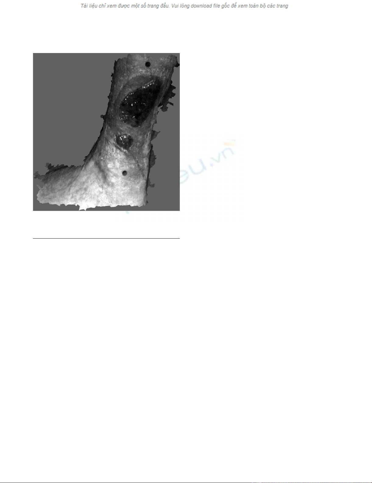
across, and are of variable depth [6,7]. Fig. 1 shows an
example of an oedemous leg infected with venous ulcers.
Published: 03 August 2005
Theoretical Biology and Medical Modelling 2005, 2:28 doi:10.1186/1742-4682-2-
28
Received: 11 May 2005
Accepted: 03 August 2005
This article is available from: http://www.tbiomed.com/content/2/1/28
© 2005 Ugail and Wilson; licensee BioMed Central Ltd.
This is an Open Access article distributed under the terms of the Creative Commons Attribution License (http://creativecommons.org/licenses/by/2.0),
which permits unrestricted use, distribution, and reproduction in any medium, provided the original work is properly cited.
Theoretical Biology and Medical Modelling 2005, 2:28 http://www.tbiomed.com/content/2/1/28
Page 2 of 9
(page number not for citation purposes)
An important task, during the treatment of oedema and
venous ulcers, is the measurement of the amount of
oedema as well as the area and volume of the ulcer
wounds. This is because without an accurate and objective
means of measuring changes in the size or shape of ulcers,
it is difficult or impossible to evaluate the efficiency of the
available therapies properly. Therefore, a prerequisite for
this development is a reliable method of measuring
ulcers. There exist a variety of measurement methods
none of which is ideal. At present direct contacting meas-
urements are widely used but they are not accurate, carry
a risk of infection and are, to say the least, uncomfortable
for the patient. For example, conventional techniques for
measuring the area and volume of wounds depend on
making physical contact with the wound, for example by
drawing around the periphery on an acetate sheet or by
making an alginate cast of the wound [6]. There is cur-
rently significant interest in developing non-invasive
measurement systems using optical methods such as
'structured light' (a technique that projects stripes on to a
surface and infers the shape from changes in the linearity
of the reflected stripe) [8] or stereo-photogrammetry. The
availability of high-resolution 3D digital cameras, increas-
ing computing power and the development of software
techniques for manipulating three-dimensional informa-
tion have benefited this area. However, equipment associ-
ated with these sorts of measurement methods is not
often portable and is often costly, thus making it prohibi-
tive for routine medical use.
The aim of this paper is to show how it is possible to
develop a system for measuring the shape and size of
limbs and venous ulcers by means of utilising an econom-
ical mathematical model. In particular, one of the out-
comes we hope to achieve from this work is a technique
with potential for clinical use. For this, a small number of
key measurements of limbs (with minimal possible con-
tact with the limb and the associated ulcer), made using
readily available instruments such as callipers and tape
measures, can be input to a computer program. The pro-
gram will then be able to reconstruct a good estimate of
the limb shape and dimensions. It is believed that such a
technique will provide a cheap, efficient, non-invasive
instrument for measuring the degree of oedema and con-
sequently enabling various treatment plans to be
evaluated.
At present there exists a wide variety of methods that can
be utilised to generate the geometry of limbs affected by
oedema and venous ulcers. These include boundary based
methods such as polygon based design [9], extrusions and
surface of revolution [10] and polynomial patches [11];
procedural modelling such as implicit surfaces [12] and
fractals [13]; and volumetric models such as constructive
solid geometry [14] and subdivision [15]. Many of these
techniques, especially polygon based design and polyno-
mial patches, would be very appropriate for limb shape
reconstruction, although they may not be ideally suited
for the problem we address here. For example, conven-
tional spline patches would require a large array of control
points and weights in order to represent a realistic shape
of a limb and associated wounds.
In this initial stage of the work we are concerned with
developing efficient techniques in order to perform two
important tasks. They are: the generation of smooth sur-
faces resembling the surface data obtained from a 3D
scanner; and, once a smooth surface is obtained, manipu-
lation of the geometry so as to obtain a good representa-
tion of the limb shape for any given patient. To do this we
utilise real data from a series of surface scans provided by
a medical partner namely, the Department of Medical
Physics and Vascular Surgery of Bradford Teaching Hospi-
tals National Health Services Trust (BTHNHST), UK, with
whom we work closely on these problems. The depart-
ment of Medical Physics at BTHNHST acquired the surface
data using multiple-camera photogrammetry with a
DSP400 system from 3dMD Ltd. This commercial tech-
nology has been widely used for acquiring medical
images, especially in the USA, and captures data in a few
An example of an oedemous leg infected with oedema venous ulcersFigure 1
An example of an oedemous leg infected with oedema
venous ulcers.

Theoretical Biology and Medical Modelling 2005, 2:28 http://www.tbiomed.com/content/2/1/28
Page 3 of 9
(page number not for citation purposes)
milliseconds. The surface resolution (i.e. the separation of
data points) is approximately 2 mm with a positional
accuracy of approximately 0.2 mm. When developing our
PDE based techniques for modelling human limbs, which
are affected by oedema and venous ulcers, our medical
partner has two aims. Firstly they require a compact and
smooth surface representation of their captured data. Sec-
ondly, and rather more importantly, they require a mod-
elling tool that would enable them to manipulate the
shape of a given limb so as to provide a good representa-
tive limb shape of any given patient.
In this paper we utilise the so called PDE method [16-18]
to address the problem. A positive feature of the PDE
method is that it can define surfaces in terms of a small set
of design variables [19], instead of many hundreds of con-
trol points. In broad terms this is because its boundary-
value approach means that PDE surfaces are defined by
data distributed around just their boundaries, instead of
data distributed over their surface area, e.g. control points.
Thus, a PDE model, when changed by altering the values
of its design parameters, remains continuous; there is no
need for a designer to intervene in order to close up any
holes that might appear at patch boundaries. In the
present context, this means that PDE surfaces can be made
to adapt to changes in the shape of the limb and the asso-
ciated wounds.
2 PDE Surfaces
A PDE surface is a parametric surface patch ,
defined as a function of two parameters u and v on a finite
domain Ω (⊂) R2 by regarding the function as a map-
ping of a point in Ω to a point in the physical
space. The shape of the surface patch is usually deter-
mined by specifying a set of boundary data at the edge of
(∂)Ω. Typically the boundary data are specified in the
form of and a number of its derivatives on (∂)Ω.
Hence, by casting the surface generation as a boundary
value problem, the surface is regarded as a solu-
tion of an elliptic PDE.
Various elliptic PDEs could be used; the ones we utilise for
this work are based on the biharmonic and triharmonic
equations, namely,
and
Also, periodic boundary conditions are very often consid-
ered. Assuming we are working with the above two elliptic
PDEs, we require them to satisfy a set of 2N conditions,
where N is 2 in the case of Equation (1) and N 3 in the
case of Equation (2). The general form of these conditions
can then be written as,
X(0, v) = f1(v), (3)
X(ui, v) = gi(v), i = 2 ... 2N - 1 (4)
X(1, v) = f2N(v), (5)
where f1(v) in Equation (3) and f2N(v) in Equation (5) are
function conditions specified at u = 0 and u = 1 respec-
tively. The conditions X(ui, v) = gi(v) in Equation (4) can
take the form either
X(ui, v) = fi for 0 <ui < 1, i = 2 ... 2N - 1, (6)
or
In simpler terms the above conditions imply that for a
PDE surface patch of order 2N, we can specify two func-
tion conditions, as given in Equations (3) and (5), that
should be satisfied at the edges (at u = 0 and u = 1) of the
surface patch, and a number of function or derivative con-
ditions, as given in Equation (4), amounting to 2N – 2
conditions that the PDE should also satisfy.
2.1 Solution of the PDEs
There exist many methods for solving Equations (1) and
(2) ranging from analytic solutions to sophisticated
numerical methods. The problems we address in this
paper involve modelling of human limbs, which are
essentially closed and cylindrical, and therefore the broad
range of shapes encountered can be incorporated by solv-
ing the chosen PDEs with periodic conditions. Note here
periodic conditions imply that for the v parameter the
condition, , is satisfied. Thus, for the
work described here, we restrict ourselves to periodic con-
ditions and obtain a closed form analytic solution of
Equations (1) and (2).
Choosing the parametric region to be 0 ≤ u ≤ 1 and 0 ≤ v
≤ 2π, and assuming that the conditions given in Equations
(3), (4) and (5) are periodic functions, we can use the
Xuv(,)
X
Xuv(,)
Xuv(,)
Xuv(,)
∂
∂+∂
∂
=
2
2
2
2
2
01
uv
Xuv(,) , ()
∂
∂+∂
∂
=
2
2
2
2
3
02
uv
Xuv(,) . ()
XXX
(,) , , , . ()uv
uu
ui N
i
N
Ni
=∂
∂
∂
∂≤≤ = −
−
−
……
22
22
01221 7for
Xu Xu(,) (, )02=
π
Theoretical Biology and Medical Modelling 2005, 2:28 http://www.tbiomed.com/content/2/1/28
Page 4 of 9
(page number not for citation purposes)
method of separation of variables and spectral approxi-
mation [20] to write down the analytic solution of Equa-
tions (1) and (2) as,
where is a polynomial function and
and are exponential functions. The specific forms
of and for the case of Equa-
tions (1) can be found in [17] and for the case of Equa-
tions (2) can be found in [21].
The main point to bear in mind regarding the above solu-
tion method is that it enables one to represent a set of gen-
eral periodic conditions in terms of a finite M Fourier
series, where M is typically taken to be ≤ 10, whilst the
term , which acts as a correction term, enables the
conditions to be satisfied exactly. Detailed discussions of
this solution method can be found in [20].
2.2 Methods of Generating PDE Surfaces
In this section we discuss a series of examples, showing
the various methods by which PDE surfaces can be gener-
ated where the PDEs are chosen to be Equations (1) and
(2) and the conditions are taken in the format described
in Equations (3), (4) and (5).
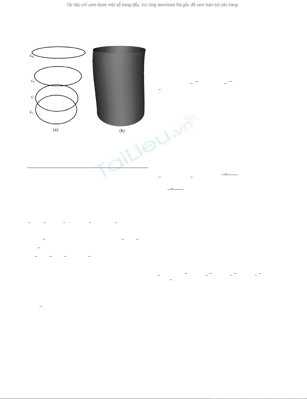
As a first example we show how a fourth order PDE sur-
face is generated where all the conditions are taken to be
function conditions. Fig. 2(b) shows the shape of a surface
generated by the fourth order PDE where the conditions
are specified in terms of the curves shown in Fig. 2(a). In
particular, the conditions are such that:
and
. Since we are taking four function condi-
tions to solve the fourth order PDE, all the curves in this
case lie on the resulting surface. Thus, in this particular
case the resulting PDE surface is a smooth interpolation
between the given set of functional conditions.
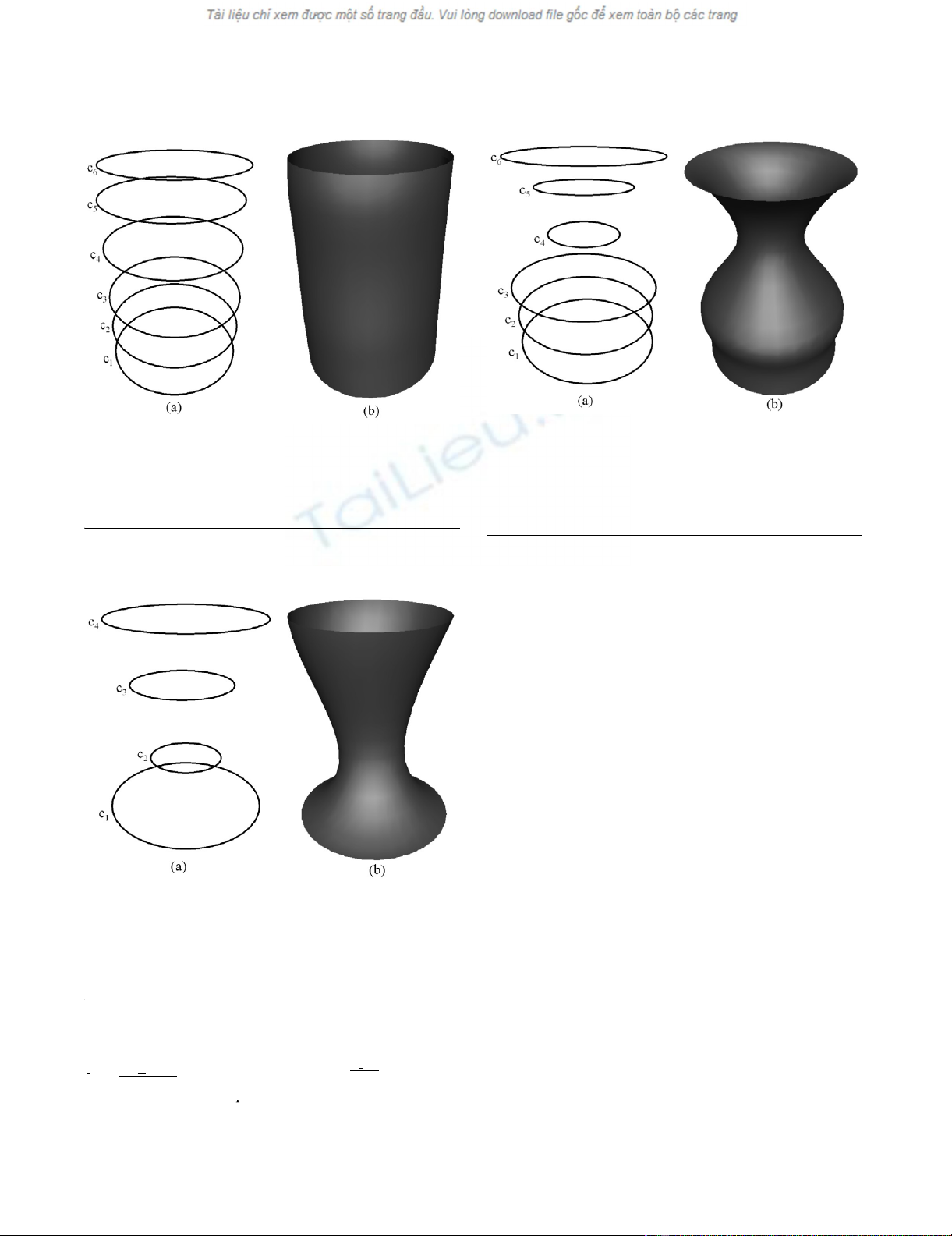
The next example shows how a fourth order PDE surface
is generated when the conditions are taken to be a mixture
of function conditions and derivative conditions. Fig.
4(b) shows the shape of a surface generated by the fourth
order PDE where two function boundary conditions and
two derivative boundary conditions are specified in terms
of the curves shown in Fig. 4(a). In particular, the bound-
ary conditions are chosen such that:
and , where s is a scalar. In this
case the surface patch generated as a solution to the fourth
order PDE contains the boundary curves c1 and c4 whilst it
does not necessarily contain the curves c2 and c3. A typical
scenario where a surface of this nature is required would
be a blend design where the derivative boundary curves
can be adjusted to produce a smooth blend surface that
bridges between two primary surfaces.
Fig. 3(b) shows the shape of a surface generated by the
sixth order PDE where the conditions are all taken to be
positions specified in terms of the curves shown in Fig.
3(a). In particular, the boundary conditions are such that
and . As in the first example of the fourth
order case, since we are taking six function conditions to
solve the sixth order PDE, all the curves in this case lie on
the resulting surface. Thus, the resulting PDE surface is a
smooth interpolation between the six prescribed curves.
As a final example we show how a sixth order PDE surface
is generated where the boundary conditions are taken to
be a mixture of function boundary conditions and deriva-
tive conditions (both first and second order). Fig. 5(b)
shows the shape of a surface generated by the sixth order
PDE where two function boundary conditions, two first
order derivative boundary conditions and two second
order derivative boundary conditions are specified in
terms of the curves shown in Fig. 5(a). In particular, the
boundary conditions are chosen such that
The shape of a surface generated by the fourth order PDE where the conditions are all taken to be function conditions (a) The conditions defined in the form of curves in 3-spaceFigure 2
The shape of a surface generated by the fourth order PDE
where the conditions are all taken to be function conditions
(a) The conditions defined in the form of curves in 3-space.
(b) The resulting surface shape.
Xuv A u A u nv B u nv Ruv
nn
n
M
(,) () [ ()cos( ) ()sin( )] (,). ()
0
1
8+++
=
∑
Au
0() AuBu
nn
(), ()
Ruv(,)
Au Au Bu
nn0(), (), () Ruv(,)
Ruv(,)
Xv cvX v cvX v cv( , ) ( ), ( , ) ( ), ( , ) ( )01
3
2
3
123
===
Xv cv(, ) ()14
=
Xv cvXv cv Xv
u
cv cvs( , ) ( ), ( , ) ( ), (,) [() ()]01 0
14 21
==
∂
∂=−
∂
∂=−
Xv
u
cv cvs
(, ) [() ()]
1
43
Xv cvX v cvX v cvX v cvX( , ) ( ), ( , ) ( ), ( , ) ( ), ( , ) ( ), (01
5
2
5
3
5
4
1234
== ==
55
5
,) ()vcv=
Xv cv(, ) ()16
=
Theoretical Biology and Medical Modelling 2005, 2:28 http://www.tbiomed.com/content/2/1/28
Page 5 of 9
(page number not for citation purposes)
and . where s and t are
scalars. As in the example of fourth order case shown in
Fig. 4 the surface generated in this case contains the curves
c1 and c6 whilst it does not necessarily contain the rest of
the curves. Again this type of surface shape can be utilised
in blend design where higher order continuity is desired
in producing a smooth blend surface that bridges between
two primary surfaces. As one can see from the format of
these derivative condition definitions, the derivative
conditions are all defined using simple finite difference
schemes. The curves defining the derivative conditions
provide an intuitive shape manipulation tool in that the
shape of the surface closely follows the shape of the
boundary conditions.
The above examples demonstrate how PDE surfaces of
order four and six can be utilised to generate surface
shapes, which are applicable to a wide variety of design
scenarios. Thus, the basic idea here is to generate a series
of curves (both function and derivative) that can be uti-
lised to define the boundary conditions for the chosen
PDE. As seen in the examples, the resulting surface shape
can always be intuitively predicted from the shapes of the
chosen curves.
3 Modelling of Limbs and Ulcers
In this section we discuss the shape modelling of human
limbs affected by oedema and venous ulcers. In what fol-
lows, we discuss two examples of shape modelling of
human limbs namely modelling of an arm shape and
modelling of a leg shape with an ulcer. We utilise a mix-
ture of PDEs of order four and six in order to model the
surface shapes in question. In order to generate a
The shape of a surface generated by the sixth order PDE where the conditions are all taken to be positions (a) The conditions defined in the form of curves in 3-spaceFigure 3
The shape of a surface generated by the sixth order PDE
where the conditions are all taken to be positions (a) The
conditions defined in the form of curves in 3-space. (b) The
resulting surface shape.
The shape of a surface generated by the fourth order PDE where the boundary conditions are taken to be both posi-tions and derivatives (a) The boundary conditions defined in the form of curves in 3-spaceFigure 4
The shape of a surface generated by the fourth order PDE
where the boundary conditions are taken to be both posi-
tions and derivatives (a) The boundary conditions defined in
the form of curves in 3-space. (b) The resulting surface
shape.
Xv cvXv cv Xv
u
cv cv s Xv
( , ) ( ), ( , ) ( ), (,) [ ( ) ( ))] , (,
01 01
16 21
==
∂
∂=− ∂)) [ ( ) ( ))] , (,) [() () ()]
∂=− ∂
∂=− +
u
cv cv s Xv
u
cv c v c vt
65
2
2123
02
∂
∂=− +
2
2645
12
Xv
u
cv cv cvt
(, ) [() () ()]
The shape of a surface generated by the sixth order PDE where the boundary conditions are taken to be both posi-tions and derivatives (a) The boundary conditions defined in the form of curves in 3-spaceFigure 5
The shape of a surface generated by the sixth order PDE
where the boundary conditions are taken to be both posi-
tions and derivatives (a) The boundary conditions defined in
the form of curves in 3-space. (b) The resulting surface
shape.


%20--%3e%3cdefs%3e%3cstyle%3e%20.st0%20{%20fill:%20%23fff;%20}%20.st1%20{%20fill:%20%237800fa;%20}%20%3c/style%3e%3c/defs%3e%3cpath%20class='st1'%20d='M117.78,12.18H43.11c2.9,3.47,4.65,7.94,4.65,12.82,0,5.6-2.3,10.66-6.01,14.29h76.02l7.22-13.56-7.22-13.56Z'/%3e%3cg%3e%3cpath%20class='st0'%20d='M53.58,26.17h-.59v-1.46h.59v-4.96h2.83c1.78,0,2.67.94,2.67,2.82v5.76c0,1.87-.89,2.81-2.67,2.81h-2.83v-4.96ZM55.36,21.37v3.34h1.1v1.46h-1.1v3.34h1.01c.61,0,.91-.37.91-1.1v-5.93c0-.74-.3-1.1-.91-1.1h-1.01Z'/%3e%3cpath%20class='st0'%20d='M65.99,31.14h-1.8l-.31-2.07h-2.19l-.31,2.07h-1.64l1.82-11.39h2.62l1.82,11.39ZM65.28,18.04c-.25.46-.51.77-.75.94-.21.15-.47.22-.79.22-.26,0-.57-.07-.92-.22l-.38-.15c-.14-.05-.26-.07-.37-.07-.3,0-.53.18-.71.54l-.91-.68c.25-.46.51-.77.75-.94.21-.14.48-.21.79-.21.26,0,.57.07.92.21l.38.15c.14.05.26.07.37.07.3,0,.53-.18.71-.54l.91.68ZM61.91,27.52h1.73l-.87-5.76-.87,5.76Z'/%3e%3cpath%20class='st0'%20d='M74.53,26.89v1.52c0,1.91-.89,2.86-2.67,2.86s-2.67-.95-2.67-2.86v-5.93c0-1.91.89-2.86,2.67-2.86s2.67.95,2.67,2.86v1.11h-1.69v-1.22c0-.75-.31-1.12-.93-1.12s-.93.37-.93,1.12v6.15c0,.74.31,1.11.93,1.11s.93-.37.93-1.11v-1.63h1.69Z'/%3e%3cpath%20class='st0'%20d='M81.4,31.14h-1.8l-.31-2.07h-2.19l-.31,2.07h-1.64l1.82-11.39h2.62l1.82,11.39ZM75.9,19.2l1.52-1.91h1.71l1.51,1.91h-1.61l-.76-.95-.75.95h-1.61ZM77.32,27.52h1.73l-.87-5.76-.87,5.76ZM83.1,15.99l-1.76,1.91h-1.26l1.17-1.91h1.86Z'/%3e%3cpath%20class='st0'%20d='M84.86,19.75c1.78,0,2.67.94,2.67,2.82v1.48c0,1.87-.89,2.81-2.67,2.81h-.85v4.28h-1.79v-11.39h2.64ZM84.01,21.37v3.86h.85c.58,0,.87-.36.87-1.08v-1.71c0-.71-.29-1.07-.87-1.07h-.85Z'/%3e%3cpath%20class='st0'%20d='M93.51,19.75c1.78,0,2.67.94,2.67,2.82v1.48c0,1.87-.89,2.81-2.67,2.81h-.85v4.28h-1.79v-11.39h2.64ZM92.66,21.37v3.86h.85c.58,0,.87-.36.87-1.08v-1.71c0-.71-.29-1.07-.87-1.07h-.85Z'/%3e%3cpath%20class='st0'%20d='M98.8,31.14h-1.79v-11.39h1.79v4.88h2.03v-4.88h1.83v11.39h-1.83v-4.88h-2.03v4.88Z'/%3e%3cpath%20class='st0'%20d='M105.36,24.55h2.46v1.62h-2.46v3.34h3.09v1.63h-4.88v-11.39h4.88v1.63h-3.09v3.18ZM108.17,17.29l-1.76,1.91h-1.26l1.17-1.91h1.86Z'/%3e%3cpath%20class='st0'%20d='M112.2,19.75c1.78,0,2.67.94,2.67,2.82v1.48c0,1.87-.89,2.81-2.67,2.81h-.85v4.28h-1.79v-11.39h2.64ZM111.35,21.37v3.86h.85c.58,0,.87-.36.87-1.08v-1.71c0-.71-.29-1.07-.87-1.07h-.85Z'/%3e%3c/g%3e%3ccircle%20class='st1'%20cx='25'%20cy='25'%20r='20'/%3e%3cpath%20class='st0'%20d='M32.78,19.27c2.92,0,4.43,2.55,5.28,5.33l.71,2.17c.14.38-.33.75-.71.75h-5.61c.19-.33.24-.71.09-1.08l-.75-2.45c-.43-1.32-.99-2.64-1.79-3.77.75-.57,1.65-.94,2.78-.94h0ZM25,18.38c3.25,0,4.9,2.78,5.89,5.89l.76,2.45c.14.42-.33.8-.8.8h-11.69c-.42,0-.94-.38-.8-.8l.75-2.45c.99-3.11,2.64-5.89,5.89-5.89h0ZM25,11.35c1.74,0,3.11,1.37,3.11,3.11s-1.37,3.11-3.11,3.11-3.11-1.41-3.11-3.11,1.41-3.11,3.11-3.11h0ZM17.27,19.27c1.08,0,1.98.38,2.73.94-.8,1.13-1.37,2.45-1.74,3.77l-.8,2.45c-.14.38-.05.75.09,1.08h-5.56c-.42,0-.9-.38-.75-.75l.71-2.17c.9-2.78,2.41-5.33,5.33-5.33h0ZM17.27,12.91c1.51,0,2.78,1.27,2.78,2.83s-1.27,2.83-2.78,2.83-2.83-1.27-2.83-2.83,1.27-2.83,2.83-2.83h0ZM32.78,12.91c1.56,0,2.78,1.27,2.78,2.83s-1.23,2.83-2.78,2.83-2.83-1.27-2.83-2.83,1.27-2.83,2.83-2.83h0ZM27.07,28.56v.09c0,.57-.24,1.08-.61,1.46h0v.05c-.38.33-.9.57-1.46.57s-1.08-.24-1.46-.61h0c-.38-.38-.61-.9-.61-1.46v-.09h1.41v.09c0,.19.05.38.19.47v.05c.09.09.28.19.47.19s.38-.09.47-.19v-.05c.14-.09.24-.28.24-.47t-.05-.09h1.41ZM30.99,28.56v.09c0,1.65-.66,3.16-1.74,4.24-1.08,1.08-2.59,1.79-4.24,1.79s-3.16-.71-4.24-1.79l-.05-.05c-1.04-1.08-1.7-2.55-1.7-4.2v-.09h1.41v.09c0,1.27.47,2.4,1.27,3.25h.05c.85.85,1.98,1.37,3.25,1.37s2.4-.52,3.25-1.37c.85-.8,1.37-1.98,1.37-3.25v-.09h1.37ZM34.99,28.56v.09c0,2.78-1.13,5.28-2.92,7.07-1.79,1.79-4.29,2.92-7.07,2.92s-5.23-1.13-7.07-2.92c-1.79-1.79-2.92-4.29-2.92-7.07v-.09h1.41v.09c0,2.4.94,4.53,2.5,6.08,1.56,1.56,3.72,2.5,6.08,2.5s4.52-.94,6.08-2.5c1.56-1.56,2.5-3.68,2.5-6.08v-.09h1.41Z'/%3e%3c/svg%3e)