1080
CHAPTER
20.
IXFORlI.4TION IXTEGRATIO-\-
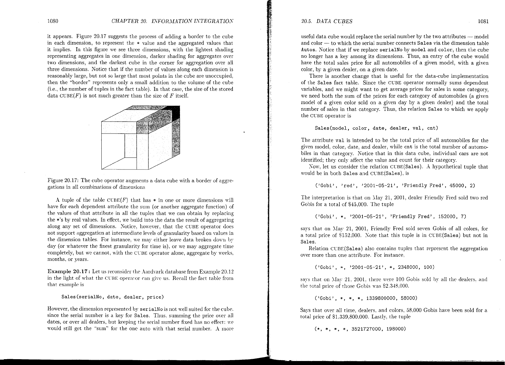
it appears. Figure 20.17 suggests the process of adding a border to the cube
in each dimension, to represent the
*
ulue and the aggregated values that
it implies. In this figure u;e see three din~ensions. with the lightest shading
representing aggregates in one dimension, darker shading for aggregates over
two dimensions, and tlle darkest cube in the corner for aggregation over all
three dimensions. Notice that if the number of values along each dirnension is
reasonably large, but not so large that most poil~ts in tlle cube are unoccupied.
then the "border" represents only a small addition to the volume of the cube
(i.e., the number of tuples in the fact table).
In
that case, the size of the stored
data
CCBE(F)
is not much greater than tlic size of
F
itself.
Figure 20.17: The cube operator augments a data cube with
a
border of aggre-
gations in all combinations of ctinien.ions
A
tuple of the table
CLBE;(F)
that has
*
in one or more dimensions TI-ill
have for each dependent attribute the sum (or another aggregate f~~nction) of
the values of that attribute in all the tuples that xve can obtain by replacing
the *'s by real values.
In
effect.
we
build into the data the result of aggregating
along any set of dimensions. Sotice. holvever. that the
CUBE
operator does
not support <\ggregation at intermediate levels of granularity based on values in
the dirnension tables For instance. ne may either leave data broken dovi-11 by
day (or whatever the finest granularity for time is). or xve may aggregate time
completely, but \re cannot, with thc
CCBE
operator alone, aggregate by weeks.
months. or years.
Example
20.17
:
Let us reconsider the -1ardvark database from Esarnple 20.12
in the light of ~vhat the
Ct-BE
oprr;i~or
can
givc us. Recall the fact table from
that exiumplc, is
Sales(serialN0, date, dealer, price)
Hoxvever, the dimension represented by
serialNo
is not well suited for the cube.
since the serial number is a key for
Sales.
Thus. sumning the price over all
dates, or over all dealers, but keeping the serial ~lumbrr fixed has
110
effect:
n-e
n-ould still gct the "sum" for the one auto ~vith that serial number.
.I
Illole
useful data cube would replace the serial number by the txo attributes
-
model
and color
-
to which the serial number connects
Sales
via the dimension table
Autos.
Sotice that if we replace
serialNo
by
model
and
color,
then tile cube
no longer has a key among its dimensions. Thus, an entry of the cube ~vould
hare the total sales price for all automobiles of a given model. with a given
color, by a given dealer, on a given date.
There is another change that is useful for the data-cube implementation
of the
Sales
fact table. Since the
CUBE
operator normally sums dependent
variables, and
13-e
might want to get average prices for sales in some category,
n-e need both the sum of the prices for each category of automobiles (a given
model of a given color sold on a given day by a given dealer) and the total
number of sales in that category. Thus, the relation
Sales
to which we apply
the
CCBE
operator is
Sales(mode1, color, date, dealer, val, cnt)
The attribute
val
is intended to be the total price of all automobiles for the
given model, color. date. and dealer, while
cnt
is the total number of automo-
biles in that category. Xotice that in this data cube. individual cars are not
identified: they only affect the value and count for their category.
Son-. let us consider the relation
cC~~(Sa1es).
.-I
hypothetical tuple that
n-ould be in both
Sales
and
ti lo sales).
is
('Gobi', 'red', '2001-05-21', 'Friendly Fred', 45000, 2)
The interpretation is that
on
May 21; 2001. dealer Friendly Fled sold two red
Gobis for a total of $45.000. The tuple
('Gobi',
*,
'2001-05-21', 'Friendly Fred', 152000,
7)
says that on SIay 21, 2001. Friendly Fred sold seven Gobis of all colors, for
a total price of S152.000. Sote that this tuple is in
sales)
but not in
Sales.
Relation
sales)
also contains tuples that represent the aggregation
over more than one attribute. For instance.
('Gobi',
*,
'2001-05-21',
*,
2348000, 100)
says rliat on \la!- 21. 2001. rllei-e n-ere 100 Gobis sold
by
all the dealers. and
the total price of tliose Gobis Tvas S2.348.000.
('Gobi',
*,
*,
*,
1339800000, 58000)
Says that over all time, dealers. and colors. 58.000 Gobis have been sold for a
total price of S1.339.800.000. Lastly. the tuple
Please purchase PDF Split-Merge on www.verypdf.com to remove this watermark.
tells us that total sales of all Aardvark lnodels in all colors, over all time at all
dealers is 198.000 cars for
a
total price of $3,521,727,000.
Consider how to answer
a
query in \\-hich we specify conditions on certain
attributes of the Sales relation and group by some other attributes, n-hile
asking for the sum, count, or average price. In the relation
are r sales),
we
look for those tuples
t
with the fo1lov;ing properties:
1. If the query specifies
a
value
v
for attribute
a;
then tuple
t
has
v
in its
component for
a.
2. If the query groups by an attribute
a,
then
t
has any non-* value in its
conlponent for
a.
3.
If the query neither groups by attribute
a
nor specifies a value for
a.
then
t
has
*
in its component for
a.
Each tuple
t
has tlie sum and count for one of the desired groups. If n-e \%-ant
the average price, a division is performed on the sum and count conlponents of
each tuple
t.
Example
20.18
:
The query
SELECT color, AVG(price)
FROM Sales
WHERE model
=
'Gobi'
GROUP
BY
color;
is ansn-ered by looking for all tuples of
sales)
~vith the form
('Gobi',
C.
*,
*,
21,
n)
here
c
is any specific color. In this tuple,
v
will be the sum of sales of Gobis
in that color, while
n
will be the nlini!)cr of sales of Gobis in that color. Tlie
average price. although not an attribute of Sales or
sales)
directly. is
v/n.
Tlie answer to the query is the set of
(c,
vln)
pairs obtained fi-om all
('Gobi'.
c,
*,
*.
v.
n)
tuples.
20.5.2
Cube ImplementaOion
by
Materialized Views
11%
suggested in Fig. 20.17 that adding
aggregations
to the cube doesn't cost
much in tcrms of space. and saves a lot in time \vhen the common kincis of
decision-support queries are asked. Ho~vever: our analysis is based on the as-
sumption that queries choose either to aggregate completely in a dimension
or not to aggregate at all. For some dime~isions. there are many degrees of
granularity that could be chosen for a grouping on that dimension.
Uc have already mentioned thc case of time. xvl-here numerolls options such
as aggregation by weeks, months: quarters, or ycars exist,, in addition to the
all-or-nothing choices of grouping by day or aggregating over all time. For
another esanlple based on our running automobile database, Ive could choose
to aggregate dealers completely or not aggregate them at all. Hon-ever, we could
also choose to aggregate by city, by state, or perhaps by other regions, larger
or smaller. Thus: there are at least sis choices of grouping for time and at least
four for dealers.
l\Tllen the number of choices for grouping along each dimension grows, it
becomes increasingly expensive to store the results of aggregating by every
possible conlbination of groupings. Sot only are there too many of them, but
they are not as easily organized as the structure of Fig. 20.17 suggests for tlle
all-or-nothing case. Thus, commercial data-cube systems may help the user to
choose some
n~aterialized
views
of the data cube.
A
materialized view is the
result of some query, which we choose to store in the database, rather than
reconstructing (parts of) it as needed in response to queries. For the data cube,
the vie~vs we n-ould choose to materialize xi11 typically be aggregations of the
full data cube.
The coarser the partition implied by the grouping, the less space the mate-
rialized view takes. On the other hand, if ire ~vant to use a view to answer a
certain query, then the view must not partition any dimension more coarsely
than the query does. Thus, to maximize the utility of materialized views, we
generally n-ant some large \-iers that group dimensions into a fairly fine parti-
tion. In addition, the choice of vien-s to materialize is heavily influenced by the
kinds of queries that the analysts are likely
to
ask.
.in
example will suggest tlie
tradeoffs in\-011-ed.
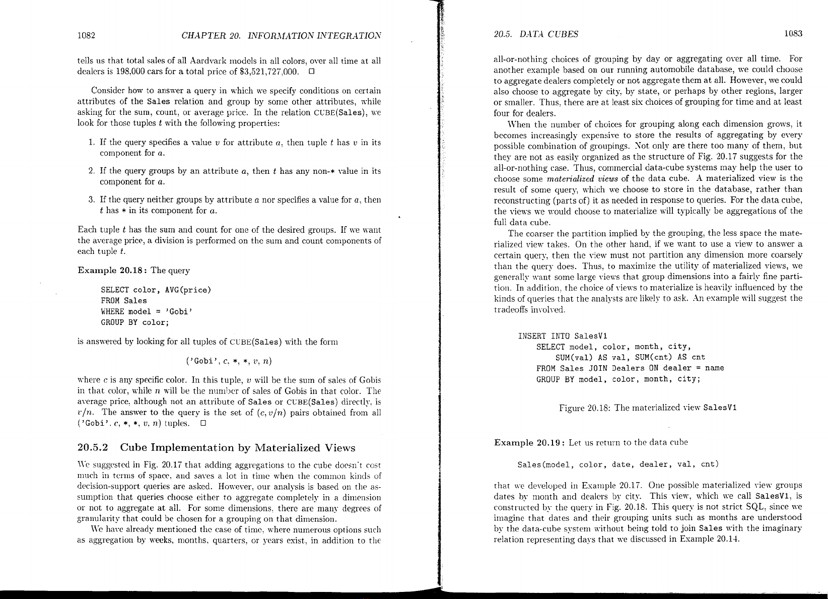
INSERT INTO SalesVl
SELECT model, color, month, city,
SUM(va1) AS val, SUM(cnt) AS cnt
FROM Sales JOIN Dealers
ON
dealer
=
name
GROUP
BY
model, color, month, city;
Figure 20.18: The materialized vien. SalesVl
Example
20.19
:
Let us return to the data cube
Sales (model, color, date, dealer, val
,
cnt)
that ne de\-eloped in Esample 20.17. One possible materialized vie\\- groups
dates by nionth and dealers by city. This view. 1%-hich
1%-e
call SalesV1, is
constlucted
by
the query in Fig. 20.18. This query is not strict
SQL.
since n-e
imagine that dates and their grouping units such as months are understood
by the data-cube system n-ithout being told to join Sales with the imaginary
relation rep~esenting dajs that \ve discussed in Example 20.14.
Please purchase PDF Split-Merge on www.verypdf.com to remove this watermark.
CHAPTER
20.
IiYFORI\IATIOAr IArTEGR.4TION
20.5.
DdT.4 CUBES
1055
INSERT INTO SalesV2
SELECT model, week, state,
SUM(va1) AS val, SUM(cnt) AS cnt
FROM Sales JOIN Dealers
ON
dealer
=
name
GROUP
BY
model, week, state;
Figure 20.19: Another materialized view,
SalesV2
Another possible materialized view aggregates colors completely, aggregates
time into u-eeks, and dealers by states. This view,
SalesV2,
is defined by the
query in Fig. 20.19. Either view
SalesVl
or
SalesV2
can be used to ansn-er a
query that partitions no more finely than either in any dimension. Thus, the
query
41:
SELECT model, SUM(va1)
FROM Sales
GROUP
BY
model;
can be answered either by
SELECT model, SUM(va1)
FROM SalesVl
GROUP
BY
model;
SELECT model, SUM(va1)
FROM SalesV2
GROUP BY model;
On the other hand, the query
42: SELECT model, year, state, SUM(va1)
FROM Sales JOIN Dealers
ON
dealer
=
name
GROUP
BY
model, year, state;
can on1 be ans\vered from
SalesV1.
as
SELECT model, year, state, SUM(va1)
FROM SalesVl
GROUP
BY
model, year, state;
Incidentally. the query inmediately above. like the qu'rics that nggregate time
units, is not strict
SQL.
That is.
state
is not ari attribute of
SalesVl:
only
city
is. \Ye rmust assume that the data-cube systenl knol\-s how to perform the
aggregation of cities into states, probably by accessing the dimension table for
dealers.
\Ye
cannot answer Q2 from
SalesV2.
Although we could roll-up cities into
states (i.e.. aggregate the cities into their states) to use
SalesV1,
we
carrrlot
roll-up ~veeks into years, since years are not evenly divided into weeks. and
data from a week beginning. say, Dec.
29,
2001. contributes to years 2001 and
2002 in a way we carinot tell from the data aggregated by weeks.
Finally, a query like
43:
SELECT model, color, date, ~~~(val)
FROM Sales
GROUP BY model, color, date;
can be anslvered from neither
SalesVl
nor
SalesV2.
It cannot be answered
from
Salesvl
because its partition of days by ~nonths is too coarse to recover
sales by day, and it cannot be ans~vered from
SalesV2
because that view does
not group by color. We would have to answer this query directly from the full
data cube.
20.5.3
The Lattice
of
Views
To formalize the cbservations of Example 20.10. it he!ps to think of a lattice of
possibl~ groupings for each dimension of the cube. The points of the lattice are
the ways that we can partition the ~alucs of a dimension
by
grouping according
to one or more attributes of its dimension table.
nB
say that partition
PI
is
belo~v partition
P2.
written
PI
5
P2
if and only if each group of
Pl
is contained
within some group of
PZ.
All
Years
/
1
I
Quarters
I
Weeks Months
Days
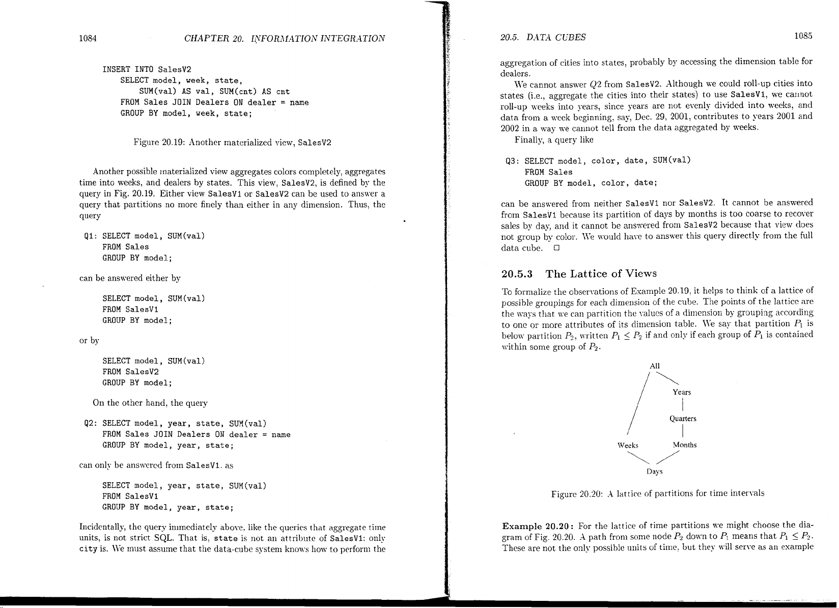
Figure 20.20:
A
lattice of partitions for time inter\-als
Example
20.20:
For the lattice of time partitions n-e might choose the dia-
gram of Fig. 20.20.
-4
path from some node
fi
dotvn to
PI
means that
PI
5
4.
These are not the only possible units of time, but they
\\-ill
serve as an example
Please purchase PDF Split-Merge on www.verypdf.com to remove this watermark.
of what units a s~stern might support. Sotice that daks lie below both \reeks
and months, but weeks do not lie below months. The reason is that while a
group of events that took place in one day surely took place within one \reek
and within one month. it is not true that a group of events taking place in one
week necessarily took place in any one month. Similarly, a week's group need
not be contained within the group cor~esponding to one quarter or to one year.
At
tlie top is a partition we call "all," meaning that events are grouped into a
single group; i.e.. we niake no distinctions among diffeient times.
All
I
State
I
City
I
Dealer
Figure 20.21:
A
lattice of partitions for automobile dealers
Figure 20.21 shows another lattice, this time for the dealer dimension of our
automobiles example. This lattice is siniplcr: it shows that partitioning sales by
dealer gives a finer partition than partitioning by the city of the dealer. i<-hich is
in turn finer than partitioning by tlie state of tlie dealer. The top of tlle ldrtice
is the partition that places all dealers in one group.
Having a lattice for each dimension,
15-12
can now define a lattice for all the
possible materialized views of a data cube that can be formed by grouping
according to some partition in each dimension. If
15
and
1%
are two views
formed by choosing a partition (grouping) for each dimension, then
1;
5
11
means that in each dimension, the partition
Pl
that ~ve use in
1;
is at least as
fine as the partition
Pl
that n.e use for that dimension in
Ti;
that is.
Pl
5
P?
Man) OLAP queries can also be placed in the lattice of views
In
fact. fie-
quently an OLAP query has the same form as the views we have described: the
query specifies some pa~titioning (possibly none or all) for each of the dimen-
sions. Other OL.iP queiics involve tliis same soit of grouping, and then "slice
tlie cube to focus
011
a subset of the data. as nas suggested
by
the diag~ani in
Fig. 20.15. The general rule is.
I\c can ansn-er a quciy
Q
using view
1-
if and o~ily if
1-
5
Q.
Example 20.21
:
Figure 20.22 takes the vielvs and queries of Example 20.19
and places them in a lattice. Sotice that the Sales data cube itself is technically
a view. corresponding to tlie finest possible partition along each climensio~l. As
we observed in the original example,
QI
can be ans~vered from either SalesVl or
Sales
Figure 20.22: The lattice of views and queries from Example 20.19
SalesV2; of course it could also be answered froni the full data cube Sales, but
there is no reason to want to do so if one of the other views is materialized.
Q2
can be answered from either SalesVl or Sales, while
Q3
can only be answered
from Sales. Each of these relationships is expressed in Fig. 20.22 by the paths
downxard from the queries to their supporting vie~vs.
Placing queries in the lattice of views helps design data-cube databases.
Some recently developed design tools for data-cube systems start with a set of
queries that they regard as ..typical" of the application at hand. They then
select
a
set of views to materialize so that each of these queries is above at least
one of the riel\-s, preferably identical to it or very close (i.e., the query and the
view use the same grouping in most of the dimensions).
20.5.4
Exercises
for
Section
20.5
Exercise 20.5.1
:
IVhat is the ratio of the size of CCBE(F) to the size of
F
if
fact table
F
has the follorving characteristics?
*
a)
F
has ten dimension attributes, each with ten different values.
b)
F
has ten dimension attributes. each with two differcnt values.
Exercise 20.5.2:
Let us use the cube ~nBE(Sa1es) from Example 20.17,
~vhich was built from the relation
Sales (model, color, date, dealer, val,
cnt)
Tcll I\-hat tuples of the cube n-e 15-ould use to answer tlle follon-ing queries:
*
a) Find the total sales of I~lue cars for each dealer.
b) Find the total nurnber of green Gobis sold by dealer .'Smilin' Sally."
c) Find the average number of Gobis sold on each day of March, 2002 by
each dealer.
Please purchase PDF Split-Merge on www.verypdf.com to remove this watermark.
1088
CHAPTER
20.
ISFORJlATIOS IXTEGRA4TIOS
*!
Exercise
20.5.3:
In Exercise 20.4.1 lve spoke of PC-order data organized as
a cube. If we are to apply the CCBE operator, we might find it convenient to
break several dimensions more finely. For example, instead of one processor
dimension, we might have one dimension for the type (e.g., AlID Duron or
Pentium-IV), and another d~mension for the speed. Suggest a set of dimrnsions
and dependent attributes that will allow us to obtain answers to a variety of
useful aggregation queries. In particular, what role does the customer play?
.Also, the price in Exercise 20.4.1 referred to the price of one macll~ne, while
several identical machines could be ordered in a single tuple. What should the
dependent attribute(s) be?
Exercise
20.5.4
:
What tuples of the cube from Exercise 20.5.3 would you use
to answer the following queries?
a) Find, for each processor speed, the total number of computers ordered in
each month of the year 2002.
b) List for each type of hard disk (e.g., SCSI or IDE) and eacli processor
type the number of computers ordered.
c) Find the average price of computers with 1500 megahertz processors for
each month from Jan., 2001.
!
Exercise
20.5.5
:
The computers described in the cube of Exercise 20.5.3 do
not include monitors. IVhat dimensions would you suggest to represent moni-
tors? You may assume that the price of the monitor is included in the price of
the computer.
Exercise
20.5.6
:
Suppose that a cube has 10 dimensions. and eacli dimension
has
5
options for granularity of aggregation. including "no aggregation" and
"aggregate fully.'' How many different views can we construct by clioosing a
granularity in each dinlension?
Exercise
20.5.7
:
Show how to add the following time units to the lattice of
Fig. 20.20: hours, minutes, seconds, fortnights (two-week periods). decades.
and centuries.
Exercise
20.5.8:
How 15-onld you change the dealer lattice of Fig. 20.21 to
include -regions." ~f:
a)
A
region is a set of states.
*
b) Regions are not com~liensurate with states. but each city is in only one
region.
c) Regions are like area codes: each region is contained \vithin a state. some
cities are in two or more regions. and some regions ha~e several cities.
20.6.
DATA
-111-YIA-G
1089
!
Exercise
20.5.9:
In Exercise 20.5.3 ne designed a cube suitable for use ~vith
the CCBE operator.
Horn-ever.
some of the dimensions could also be given a non-
trivial lattice structure. In particular, the processor type could be organized by
manufacturer (e
g., SUT, Intel. .AND. llotorola). series (e.g..
SUN
Ult~aSparc.
Intel Pentium or Celeron. AlID rlthlon, or llotorola G-series), and model (e.g.,
Pentiuni-I\- or G4).
a) Design tlie lattice of processor types following the examples described
above.
b) Define a view that groups processors by series, hard disks by type, and
removable disks by speed, aggregating everything else.
c) Define a view that groups processors by manufacturer, hard disks by
speed. and aggregates everything else except memory size.
d) Give esamples of qneries that can be ansn-ered from the view of (11) only,
the vieiv of (c) only, both, and neither.
*!!
Exercise
20.5.10:
If the fact table
F
to n-hicli n-e apply the
CuBE
operator is
sparse (i.e.. there are inany fen-er tuples in
F
than the product of the number
of possihle values along each dimension), then tlie ratio of the sizes of CCBE(F)
and
F
can be very large. Hon large can it be?
20.6
Data
Mining
A
family of database applications cal!ed
data
rnin,ing
or
knowledge discovery
in
dntnbases
has captured considerable interest because of opportunities to learn
surprising facts fro111 esisting databases. Data-mining queries can be thought
of as an estended form of decision-support querx, although the distinction is in-
formal (see the box on -Data-llining Queries and Decision-Support Queries").
Data nli11i11:. stresses both the cpcry-optimization and data-management com-
ponents of a traditional database system, as 1%-ell as suggesting some important
estensions to database languages, such as language primitix-es that support effi-
cient sampling of data. In this section, we shall esamine the principal directions
data-mining applications have taken. Me then focus on tlie problem called "fre-
quc'iit iteinsets." n-hich has 1-eceiwd the most attention from the database point
of view.
20.6.1
Data-Iblining Applications
Broadly. data-mining queries ask for a useful summary of data, often ~vithout
suggcstir~g the values of para~netcrs that would best yield such a summary.
This family of problems thus requires rethinking the nay database systems are
to be used to provide snch insights abo~it the data. Below are some of tlie
applications and problems that are being addressed using very large amounts
Please purchase PDF Split-Merge on www.verypdf.com to remove this watermark.


![BIOS: Những điều cần biết [A-Z]](https://cdn.tailieu.vn/images/document/thumbnail/2013/20130709/sunshine_5/135x160/1517459_259.jpg)


%20--%3e%3cdefs%3e%3cstyle%3e%20.st0%20{%20fill:%20%23fff;%20}%20.st1%20{%20fill:%20%237800fa;%20}%20%3c/style%3e%3c/defs%3e%3cpath%20class='st1'%20d='M117.78,12.18H43.11c2.9,3.47,4.65,7.94,4.65,12.82,0,5.6-2.3,10.66-6.01,14.29h76.02l7.22-13.56-7.22-13.56Z'/%3e%3cg%3e%3cpath%20class='st0'%20d='M53.58,26.17h-.59v-1.46h.59v-4.96h2.83c1.78,0,2.67.94,2.67,2.82v5.76c0,1.87-.89,2.81-2.67,2.81h-2.83v-4.96ZM55.36,21.37v3.34h1.1v1.46h-1.1v3.34h1.01c.61,0,.91-.37.91-1.1v-5.93c0-.74-.3-1.1-.91-1.1h-1.01Z'/%3e%3cpath%20class='st0'%20d='M65.99,31.14h-1.8l-.31-2.07h-2.19l-.31,2.07h-1.64l1.82-11.39h2.62l1.82,11.39ZM65.28,18.04c-.25.46-.51.77-.75.94-.21.15-.47.22-.79.22-.26,0-.57-.07-.92-.22l-.38-.15c-.14-.05-.26-.07-.37-.07-.3,0-.53.18-.71.54l-.91-.68c.25-.46.51-.77.75-.94.21-.14.48-.21.79-.21.26,0,.57.07.92.21l.38.15c.14.05.26.07.37.07.3,0,.53-.18.71-.54l.91.68ZM61.91,27.52h1.73l-.87-5.76-.87,5.76Z'/%3e%3cpath%20class='st0'%20d='M74.53,26.89v1.52c0,1.91-.89,2.86-2.67,2.86s-2.67-.95-2.67-2.86v-5.93c0-1.91.89-2.86,2.67-2.86s2.67.95,2.67,2.86v1.11h-1.69v-1.22c0-.75-.31-1.12-.93-1.12s-.93.37-.93,1.12v6.15c0,.74.31,1.11.93,1.11s.93-.37.93-1.11v-1.63h1.69Z'/%3e%3cpath%20class='st0'%20d='M81.4,31.14h-1.8l-.31-2.07h-2.19l-.31,2.07h-1.64l1.82-11.39h2.62l1.82,11.39ZM75.9,19.2l1.52-1.91h1.71l1.51,1.91h-1.61l-.76-.95-.75.95h-1.61ZM77.32,27.52h1.73l-.87-5.76-.87,5.76ZM83.1,15.99l-1.76,1.91h-1.26l1.17-1.91h1.86Z'/%3e%3cpath%20class='st0'%20d='M84.86,19.75c1.78,0,2.67.94,2.67,2.82v1.48c0,1.87-.89,2.81-2.67,2.81h-.85v4.28h-1.79v-11.39h2.64ZM84.01,21.37v3.86h.85c.58,0,.87-.36.87-1.08v-1.71c0-.71-.29-1.07-.87-1.07h-.85Z'/%3e%3cpath%20class='st0'%20d='M93.51,19.75c1.78,0,2.67.94,2.67,2.82v1.48c0,1.87-.89,2.81-2.67,2.81h-.85v4.28h-1.79v-11.39h2.64ZM92.66,21.37v3.86h.85c.58,0,.87-.36.87-1.08v-1.71c0-.71-.29-1.07-.87-1.07h-.85Z'/%3e%3cpath%20class='st0'%20d='M98.8,31.14h-1.79v-11.39h1.79v4.88h2.03v-4.88h1.83v11.39h-1.83v-4.88h-2.03v4.88Z'/%3e%3cpath%20class='st0'%20d='M105.36,24.55h2.46v1.62h-2.46v3.34h3.09v1.63h-4.88v-11.39h4.88v1.63h-3.09v3.18ZM108.17,17.29l-1.76,1.91h-1.26l1.17-1.91h1.86Z'/%3e%3cpath%20class='st0'%20d='M112.2,19.75c1.78,0,2.67.94,2.67,2.82v1.48c0,1.87-.89,2.81-2.67,2.81h-.85v4.28h-1.79v-11.39h2.64ZM111.35,21.37v3.86h.85c.58,0,.87-.36.87-1.08v-1.71c0-.71-.29-1.07-.87-1.07h-.85Z'/%3e%3c/g%3e%3ccircle%20class='st1'%20cx='25'%20cy='25'%20r='20'/%3e%3cpath%20class='st0'%20d='M32.78,19.27c2.92,0,4.43,2.55,5.28,5.33l.71,2.17c.14.38-.33.75-.71.75h-5.61c.19-.33.24-.71.09-1.08l-.75-2.45c-.43-1.32-.99-2.64-1.79-3.77.75-.57,1.65-.94,2.78-.94h0ZM25,18.38c3.25,0,4.9,2.78,5.89,5.89l.76,2.45c.14.42-.33.8-.8.8h-11.69c-.42,0-.94-.38-.8-.8l.75-2.45c.99-3.11,2.64-5.89,5.89-5.89h0ZM25,11.35c1.74,0,3.11,1.37,3.11,3.11s-1.37,3.11-3.11,3.11-3.11-1.41-3.11-3.11,1.41-3.11,3.11-3.11h0ZM17.27,19.27c1.08,0,1.98.38,2.73.94-.8,1.13-1.37,2.45-1.74,3.77l-.8,2.45c-.14.38-.05.75.09,1.08h-5.56c-.42,0-.9-.38-.75-.75l.71-2.17c.9-2.78,2.41-5.33,5.33-5.33h0ZM17.27,12.91c1.51,0,2.78,1.27,2.78,2.83s-1.27,2.83-2.78,2.83-2.83-1.27-2.83-2.83,1.27-2.83,2.83-2.83h0ZM32.78,12.91c1.56,0,2.78,1.27,2.78,2.83s-1.23,2.83-2.78,2.83-2.83-1.27-2.83-2.83,1.27-2.83,2.83-2.83h0ZM27.07,28.56v.09c0,.57-.24,1.08-.61,1.46h0v.05c-.38.33-.9.57-1.46.57s-1.08-.24-1.46-.61h0c-.38-.38-.61-.9-.61-1.46v-.09h1.41v.09c0,.19.05.38.19.47v.05c.09.09.28.19.47.19s.38-.09.47-.19v-.05c.14-.09.24-.28.24-.47t-.05-.09h1.41ZM30.99,28.56v.09c0,1.65-.66,3.16-1.74,4.24-1.08,1.08-2.59,1.79-4.24,1.79s-3.16-.71-4.24-1.79l-.05-.05c-1.04-1.08-1.7-2.55-1.7-4.2v-.09h1.41v.09c0,1.27.47,2.4,1.27,3.25h.05c.85.85,1.98,1.37,3.25,1.37s2.4-.52,3.25-1.37c.85-.8,1.37-1.98,1.37-3.25v-.09h1.37ZM34.99,28.56v.09c0,2.78-1.13,5.28-2.92,7.07-1.79,1.79-4.29,2.92-7.07,2.92s-5.23-1.13-7.07-2.92c-1.79-1.79-2.92-4.29-2.92-7.07v-.09h1.41v.09c0,2.4.94,4.53,2.5,6.08,1.56,1.56,3.72,2.5,6.08,2.5s4.52-.94,6.08-2.5c1.56-1.56,2.5-3.68,2.5-6.08v-.09h1.41Z'/%3e%3c/svg%3e)