
Advances in Natural Sciences, Vol. 7, No. 1 & 2 (2006) (1 – 12)
Physics
DYSON EQUATIONS FOR GREEN FUNCTIONS OF
ELECTRONS IN OPEN SINGLE-LEVEL QUANTUM DOT
Nguyen Van Hieu and Nguyen Bich Ha
Institute of Materials Science VAST and College of Technology VNUH
Nguyen Van Hop
Faculty of Physics, Hanoi National University of Education
Abstract. The infinite system of differential equations for the nonequilibrium Green functions
of electrons in a single-level quantum dot connected with two conducting leads is truncated by
applying the mean-field approximation to the mean values of the products of four operators. As
the result the system of Dyson equations for the two-point real-time nonequilibrium Green func-
tions in the Keldysh formalism as well as that of the two-point imaginary-time Green functions
are derived.
1. INTRODUCTION
The electrons transport through a single-level quantum dot (QD) connected with
two conducting leads was the subject for the theoretical and experimental studies in many
works since the early days of the nanophysics [1-19]. Two observable physical quantities
which can be measured in the experiments on the electrons transport are the electron
current through the QD and the time-averaged value of the electrons number in the QD.
All they are expressed in terms of the single-electron Green functions. Since the electron
transport is a nonequilibrium process one should work with the in Keldysh formalism of
nonequilibrium complex-time Green functions [20,21]. Due to the presence of the strong
Coulomb interaction between electrons in the QD the differential equations for the single-
electron Green functions contain the multi-electron Green functions and all these coupled
equations form an infinite system of differential equations for an infinite number of Green
functions. In order to find some approximate finite closed system of equations one can
either to apply the perturbation theory and retain only some appropriate chain of ladder
diagrams or to assume some approximation to decouple the infinite system of equations
and obtain a finite closed system. In the former case one should use the noncrossing
approximation. In both cases the form of the approximate finite system of equations
depends on the mechanism of the approximation and therefore the approximate systems in
different works are different. In order to prepare our further study we revise the derivation
of the approximate finite system of equations for the complex-time Green functions of
electrons in the open single-level QD. As the mechanism for decoupling the infinite system
of equations to obtain the approximate finite one we assume the mean-field approximation
to the mean values of the products of four operators. The system of two Dyson equations
for two complex-time two-point Green functions will be derived.

2Nguyen Van Hieu, Nguyen Bich Ha, and Nguyen Van Hop
In Sec. II the Hamiltonian of the model and the equations of motion for the electron
destruction and creation operators are presented. The differential equations for the Green
functions are derived in Sec. III. In Sec. IV from the mean-field approximation it follows
the relations between the Green functions which decouple the infinite system of equations
and lead to the closed system of Dyson equations for two complex-time Green functions.
The conclusion and discussions are presented in Sec. V.
2. HAMILTONIAN AND EQUATIONS OF MOTION
Consider the single electron transistor (SET) consisting of a single-level quantum dot
(QD) connected with two conducting leads through two potential barriers. The electron
transport through this SET was investigated experimentally and studied in many theoret-
ical works [1-19]. It was assumed that the electron system in this SET has following total
Hamiltonian
H=EX
σ
c+
σcσ+Un↑n↓+X
kX
σEa(k)a+
σ(k)aσ(k)+Eb(k)b+
σ(k)bσ(k)
+X
kX
σVa(k)a+
σ(k)cσ+V∗
a(k)c+
σaσ(k)+Vb(k)b+
σ(k)cσ+V∗
b(k)c+
σbσ(k),
nσ=c+
σcσ,σ=↑,↓,
E=E0−µ, Ea(k)=E0
a(k)−µa,E
b(k)=E0
b(k)−µb,
(1)
where cσand c+
σare the destruction and creation operators for the electron at the energy
level E0in the QD, aσ(k), bσ(k) and a+
σ(k), b+
σ(k) are those of the electrons with the
kinetic energies E0
a(k), E0
b(k), resp., in the leads; µ,µa,µbare the corresponding chemical
potentials, Va(k) and Vb(k) are the coupling constants in the effective tunneling interaction
Hamiltonian.
For the study of the Green functions we work in the Heisenberg picture and set
cσ(t)=eiHtcσe−iH t,¯cσ(t)=eiH tc+
σe−iHt,
aσ(k,t)=eiH taσ(k)e−iH t,¯aσ(k,t)=eiHta+
σ(k)e−iHt,(2)
bσ(k,t)=eiHtbσ(k)e−iHt,¯
bσ(k,t)=eiHtb+
σ(k)e−iHt.
These formulae can be used not only for the real time t, but also for the complex time t
in the Keldysh formalism. In terms of the operators in the l. h. s. of the formulae (2) we
define the Green functions
Gc¯c
σσ′(t−t′)=δσσ′Gc¯c(t−t′)=−iTC[cσ(t)¯cσ′(t′)]β,(3)
Hc¯c
σσ′(t−t′)=δσσ′Hc¯c(t−t′)=−iTC[n−σ(t)cσ(t)¯cσ′t′]β,(4)
Ga¯c
σσ′(k;t−t′)=δσσ′Ga¯c(k;t−t′)=−iTC[aσ(k,t)¯cσ′(t′)]β,(5)
Ha¯c
σσ′(k;t−t′)=δσσ′Ha¯c(k;t−t′)=−iTC[n−σ(t)aσ(k,t)¯cσ′(t′)]β,(6)
Gac¯c¯c
σσ′(k;t−t′)=δσσ′Gac¯c¯c(k;t−t′)=−iTC[a−σ(k,t)cσ(t)¯c−σ(t)¯cσ′t′]β,(7)
Dyson Equations for Green Functions of Electrons in Open Single-level Quantum Dot 3
Gcc¯a¯c
σσ′(k;t−t′)=δσσ′Gcc¯a¯c(k;t−t′)=−iTC[c−σ(t)cσ(t)¯a−σ(k;t)¯cσ′t′]β,(8)
Gaa¯c¯c
σσ′(k,l;t−t′)=δσσ′Gaa¯c¯c
σσ′(k,l;t−t′)=−iTC[a−σ(k,t)aσ(l,t)¯c−σ(t)¯cσ′t′]β,(9)
Gac¯a¯c
σσ′(k,l;t−t′)=δσσ′Gac¯a¯c(k,l;t−t′)=−iTC[a−σ(k,t)cσ(t)¯a−σ(l,t)¯cσ′t′]β(10)
and similarly for the others
Gb¯c
σσ′(k;t−t′),H
b¯c
σσ′(k;t−t′),G
bc¯c¯c
σσ′(k;t−t′),
Gcc¯
b¯c
σσ′(k;t−t′),G
ab¯c¯c
σσ′(k,l;t−t′),G
ac¯
b¯c
σσ′(k,l;t−t′)
etc., where h...iβdenote the thermal equilibrium statistical average value
h...iβ=Tr...e
−βH
Tr{e−βH }
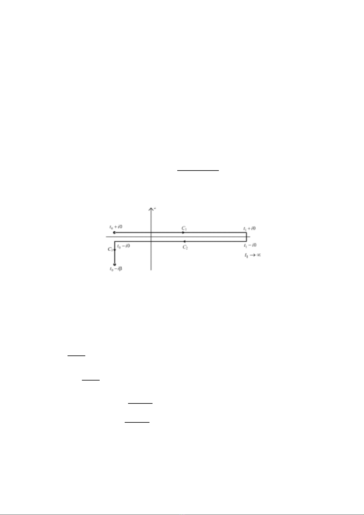
and TCdenote the ordering along the Keldysh contour C in the complex tplane presented
in Fig. 1.
Fig. 1.Contour Cconsists of three parts C=C1∪C2∪C3.
Because there is no magnetic interaction all Green functions (3)–(10) are propor-
tional to δσσ′. From the equal-time canonical anti-commutation relations between the
electron destruction and creation operators it follows the equations of motion for the
operators
idcσ(t)
dt =Ecσ(t)+Un−σ(t)cσ(t)+X
k
[V∗
a(k)aσ(k,t)+ V∗
b(k)bσ(k,t)],(11)
id¯cσ(t)
dt =−E¯cσ(t)−Un−σ(t)¯cσ(t)−X
k
[Va(k)¯aσ(k,t)+Vb(k)¯
bσ(k,t)],(12)
idaσ(k,t)
dt =Ea(k)aσ(k,t)+Va(k)cσ(t),(13)
id¯aσ(k,t)
dt =−Ea(k)¯aσ(k,t)−V∗
a(k)¯cσ(t),(14)
and similarly for bσ(k,t) and ¯
bσ(k,t).

4Nguyen Van Hieu, Nguyen Bich Ha, and Nguyen Van Hop
3. DIFFERENTIAL EQUATIONS FOR THE GREEN FUNCTIONS
Using the equation of motion (11) and the equal-time canonical anti-commutation
relation between cσ(t) and ¯cσ′(t′) it is easy to derive the differential equation for the Green
function Gc¯c
σσ′(t−t′)
id
dt −EGc¯c
σσ′(t−t′)=δσσ′δC(t−t′)+UHc¯c
σσ′(t−t′)
+X
k
[V∗
a(k)Ga¯c
σσ′(k;t−t′)+V∗
b(k)Gb¯c
σσ′(k;t−t′)],
(15)
which contains the Green functions Hc¯c
σσ′(t−t′), Ga¯c
σσ′(k;t−t′) and Gb¯c
σσ′(k;t−t′). These
new functions must satisfy following differential equations which can be also derived by
using the equations of motion (11)–(14)
id
dt −(E+U)Hc¯c
σσ′(t−t′)
=nδC(t−t′)+X
k
[V∗
a(k)Ha¯c
σσ′(k;t−t′)+V∗
b(k)Hb¯c
σσ′(k;t−t′)]
+X
khV∗
a(k)Gac¯c¯c
σσ′(k;t−t′)+V∗
b(k)Gbc¯c¯c
σσ′(k;t−t′)
−Va(k)Gcc¯a¯c
σσ′(k;t−t′)−Vb(k)Gcc¯
b¯c
σσ′(k;t−t′)i,
(16)
where
n=Dc+
↑c↑E=Dc+
↓c↓E,(17)
id
dt −Ea(k)Ga¯c
σσ′(k;t−t′)= Va(k)Gc¯c
σσ′(t−t′),(18)
and similarly for Gb¯c
σσ′(k;t−t′).
Introduce the complex-time Green function SE(t−t′) of the free electron with a
given energy E. It is the solution of the differential equation
id
dt −ESE(t−t′)= δC(t−t′).(19)
Then we can write the solution of the differential equation (18) in the integral form
Ga¯c
σσ′(k;t−t′)=Va(k)Z
C
dt′′SE(t−t′′)Gc¯c
σσ′(t−t′′),(20)
and similarly for Gb¯c
σσ′(k;t−t′).Substituting the expression of the form (20) for Ga¯c
σσ′(k;t−
t′) and Gb¯c
σσ′(k;t−t′) into the r.h.s. of the differential equation (15) for Gc¯c
σσ′(t−t′)we
rewrite this equation in the new form
id
dt −EGc¯c
σσ′(t−t′)=δσσ′δC(t−t′)+UHc¯c
σσ′(t−t′)+Z
C
dt′′Σ(1)(t−t′′)Gc¯c
σσ′(t′′−t),(21)

Dyson Equations for Green Functions of Electrons in Open Single-level Quantum Dot 5
where Σ(1)(t−t′′) is the following self-energy part
Σ(1)(t−t′)=X
kn|Va(k)|2SEa(k)(t−t′)+|Vb(k)|2SEb(k)(t−t′)o.(22)
The differential equation for the Green function Hc¯c
σσ′(t−t′) contains the Green
function Ha¯c
σσ′(k;t−t′), Hb¯c
σσ′(k;t−t′), Gac¯c¯c
σσ′(k;t−t′), Gbc¯c¯c
σσ′(k;t−t′), Gcc¯a¯c
σσ′(k;t−t′) and
Gcc¯
b¯c
σσ′(k;t−t′) which must satisfy following differential equations
id
dt −Ea(k)Ha¯c
σσ′(k;t−t′)=Va(k)Hc¯c
σσ′(t−t′),(23)
and similarly for Hb¯c
σσ′(k;t−t′),
id
dt −Ea(k)Gac¯c¯c
σσ′(k;t−t′)
=a−σ(k)cσc+
−σ,c
+
σ′δC(t−t′)+Va(k)[Hc¯c
σσ′(t−t′)−Gc¯c
σσ′(t−t′)]
+X
l
[V∗
a(l)Gaa¯c¯c
σσ′(k,l;t−t′)+V∗
b(l)Gab¯c¯c
σσ′(k,l;t−t′)]
−X
l
[Va(l)Gac¯a¯c
σσ′(k,l;t−t′)+Vb(l)Gac¯
b¯c
σσ′(k,l;t−t′)],
(24)
and similarly for Gbc¯c¯c
σσ′(k;t−t′),
id
dt −[2E−Ea(k)+U]Gcc¯a¯c
σσ′(k;t−t′)
={c−σcσa+
−σ(k),c
+
σ′}δC(t−t′)−V∗
a(k)[Hc¯c
σσ′(t−t′)−Gc¯c
σσ′(t−t′)]
+X
lV∗
a(l)[Gac¯a¯c
σσ′(l,k;t−t′)+Gca¯a¯c
σσ′(l,k;t−t′)]
+V∗
b(l)[Gbc¯a¯c
σσ′(l,k;t−t′)+Gcb¯a¯c
σσ′(l,k;t−t′)]o,
(25)
and similarly for Gcc¯
b¯c
σσ′(k;t−t′). The solutions of the differential equations (23), (24) and
(25) can be written in the integral form
Ha¯c
σσ′(k;t−t′)=Va(k)Z
C
dt′′SEa(k)(t−t′′)Hc¯c
σσ′(t′′−t′),(26)


%20--%3e%3cdefs%3e%3cstyle%3e%20.st0%20{%20fill:%20%23fff;%20}%20.st1%20{%20fill:%20%237800fa;%20}%20%3c/style%3e%3c/defs%3e%3cpath%20class='st1'%20d='M117.78,12.18H43.11c2.9,3.47,4.65,7.94,4.65,12.82,0,5.6-2.3,10.66-6.01,14.29h76.02l7.22-13.56-7.22-13.56Z'/%3e%3cg%3e%3cpath%20class='st0'%20d='M53.58,26.17h-.59v-1.46h.59v-4.96h2.83c1.78,0,2.67.94,2.67,2.82v5.76c0,1.87-.89,2.81-2.67,2.81h-2.83v-4.96ZM55.36,21.37v3.34h1.1v1.46h-1.1v3.34h1.01c.61,0,.91-.37.91-1.1v-5.93c0-.74-.3-1.1-.91-1.1h-1.01Z'/%3e%3cpath%20class='st0'%20d='M65.99,31.14h-1.8l-.31-2.07h-2.19l-.31,2.07h-1.64l1.82-11.39h2.62l1.82,11.39ZM65.28,18.04c-.25.46-.51.77-.75.94-.21.15-.47.22-.79.22-.26,0-.57-.07-.92-.22l-.38-.15c-.14-.05-.26-.07-.37-.07-.3,0-.53.18-.71.54l-.91-.68c.25-.46.51-.77.75-.94.21-.14.48-.21.79-.21.26,0,.57.07.92.21l.38.15c.14.05.26.07.37.07.3,0,.53-.18.71-.54l.91.68ZM61.91,27.52h1.73l-.87-5.76-.87,5.76Z'/%3e%3cpath%20class='st0'%20d='M74.53,26.89v1.52c0,1.91-.89,2.86-2.67,2.86s-2.67-.95-2.67-2.86v-5.93c0-1.91.89-2.86,2.67-2.86s2.67.95,2.67,2.86v1.11h-1.69v-1.22c0-.75-.31-1.12-.93-1.12s-.93.37-.93,1.12v6.15c0,.74.31,1.11.93,1.11s.93-.37.93-1.11v-1.63h1.69Z'/%3e%3cpath%20class='st0'%20d='M81.4,31.14h-1.8l-.31-2.07h-2.19l-.31,2.07h-1.64l1.82-11.39h2.62l1.82,11.39ZM75.9,19.2l1.52-1.91h1.71l1.51,1.91h-1.61l-.76-.95-.75.95h-1.61ZM77.32,27.52h1.73l-.87-5.76-.87,5.76ZM83.1,15.99l-1.76,1.91h-1.26l1.17-1.91h1.86Z'/%3e%3cpath%20class='st0'%20d='M84.86,19.75c1.78,0,2.67.94,2.67,2.82v1.48c0,1.87-.89,2.81-2.67,2.81h-.85v4.28h-1.79v-11.39h2.64ZM84.01,21.37v3.86h.85c.58,0,.87-.36.87-1.08v-1.71c0-.71-.29-1.07-.87-1.07h-.85Z'/%3e%3cpath%20class='st0'%20d='M93.51,19.75c1.78,0,2.67.94,2.67,2.82v1.48c0,1.87-.89,2.81-2.67,2.81h-.85v4.28h-1.79v-11.39h2.64ZM92.66,21.37v3.86h.85c.58,0,.87-.36.87-1.08v-1.71c0-.71-.29-1.07-.87-1.07h-.85Z'/%3e%3cpath%20class='st0'%20d='M98.8,31.14h-1.79v-11.39h1.79v4.88h2.03v-4.88h1.83v11.39h-1.83v-4.88h-2.03v4.88Z'/%3e%3cpath%20class='st0'%20d='M105.36,24.55h2.46v1.62h-2.46v3.34h3.09v1.63h-4.88v-11.39h4.88v1.63h-3.09v3.18ZM108.17,17.29l-1.76,1.91h-1.26l1.17-1.91h1.86Z'/%3e%3cpath%20class='st0'%20d='M112.2,19.75c1.78,0,2.67.94,2.67,2.82v1.48c0,1.87-.89,2.81-2.67,2.81h-.85v4.28h-1.79v-11.39h2.64ZM111.35,21.37v3.86h.85c.58,0,.87-.36.87-1.08v-1.71c0-.71-.29-1.07-.87-1.07h-.85Z'/%3e%3c/g%3e%3ccircle%20class='st1'%20cx='25'%20cy='25'%20r='20'/%3e%3cpath%20class='st0'%20d='M32.78,19.27c2.92,0,4.43,2.55,5.28,5.33l.71,2.17c.14.38-.33.75-.71.75h-5.61c.19-.33.24-.71.09-1.08l-.75-2.45c-.43-1.32-.99-2.64-1.79-3.77.75-.57,1.65-.94,2.78-.94h0ZM25,18.38c3.25,0,4.9,2.78,5.89,5.89l.76,2.45c.14.42-.33.8-.8.8h-11.69c-.42,0-.94-.38-.8-.8l.75-2.45c.99-3.11,2.64-5.89,5.89-5.89h0ZM25,11.35c1.74,0,3.11,1.37,3.11,3.11s-1.37,3.11-3.11,3.11-3.11-1.41-3.11-3.11,1.41-3.11,3.11-3.11h0ZM17.27,19.27c1.08,0,1.98.38,2.73.94-.8,1.13-1.37,2.45-1.74,3.77l-.8,2.45c-.14.38-.05.75.09,1.08h-5.56c-.42,0-.9-.38-.75-.75l.71-2.17c.9-2.78,2.41-5.33,5.33-5.33h0ZM17.27,12.91c1.51,0,2.78,1.27,2.78,2.83s-1.27,2.83-2.78,2.83-2.83-1.27-2.83-2.83,1.27-2.83,2.83-2.83h0ZM32.78,12.91c1.56,0,2.78,1.27,2.78,2.83s-1.23,2.83-2.78,2.83-2.83-1.27-2.83-2.83,1.27-2.83,2.83-2.83h0ZM27.07,28.56v.09c0,.57-.24,1.08-.61,1.46h0v.05c-.38.33-.9.57-1.46.57s-1.08-.24-1.46-.61h0c-.38-.38-.61-.9-.61-1.46v-.09h1.41v.09c0,.19.05.38.19.47v.05c.09.09.28.19.47.19s.38-.09.47-.19v-.05c.14-.09.24-.28.24-.47t-.05-.09h1.41ZM30.99,28.56v.09c0,1.65-.66,3.16-1.74,4.24-1.08,1.08-2.59,1.79-4.24,1.79s-3.16-.71-4.24-1.79l-.05-.05c-1.04-1.08-1.7-2.55-1.7-4.2v-.09h1.41v.09c0,1.27.47,2.4,1.27,3.25h.05c.85.85,1.98,1.37,3.25,1.37s2.4-.52,3.25-1.37c.85-.8,1.37-1.98,1.37-3.25v-.09h1.37ZM34.99,28.56v.09c0,2.78-1.13,5.28-2.92,7.07-1.79,1.79-4.29,2.92-7.07,2.92s-5.23-1.13-7.07-2.92c-1.79-1.79-2.92-4.29-2.92-7.07v-.09h1.41v.09c0,2.4.94,4.53,2.5,6.08,1.56,1.56,3.72,2.5,6.08,2.5s4.52-.94,6.08-2.5c1.56-1.56,2.5-3.68,2.5-6.08v-.09h1.41Z'/%3e%3c/svg%3e)