Academic Editors: Seyed
Morteza Alizadeh and Akhtar Kalam
Received: 28 May 2025
Revised: 5 July 2025
Accepted: 7 July 2025
Published: 10 July 2025
Citation: Shu, H.; Nguyen, L.M.T.;
Nguyen, X.V.; Doan, Q.H. Fault
Location on Three-Terminal
Transmission Lines Without Utilizing
Line Parameters. Electricity 2025,6, 42.
https://doi.org/10.3390/
electricity6030042
Copyright: © 2025 by the authors.
Licensee MDPI, Basel, Switzerland.
This article is an open access article
distributed under the terms and
conditions of the Creative Commons
Attribution (CC BY) license
(https://creativecommons.org/
licenses/by/4.0/).
Article
Fault Location on Three-Terminal Transmission Lines Without
Utilizing Line Parameters
Hongchun Shu 1, Le Minh Tri Nguyen 1,2,* , Xuan Vinh Nguyen 2and Quoc Hung Doan 2
1Faculty of Electrical Power Engineering, Kunming University of Science and Technology,
Kunming 650051, China; kmshc@sina.com
2Faculty of Electrical and Electronics Engineering, Vinh Long University of Technology and Education,
Vinh Long 89000, Vietnam; vinhnx@vlute.edu.vn (X.V.N.); dqhung@kgc.edu.vn (Q.H.D.)
*Correspondence: nlmtri@kgc.edu.vn; Tel.: +86-18860743709
Abstract
Transmission lines are constantly exposed to changes in climatic conditions and aging
which affect the parameters and change the characteristics of the three-terminal circuit over
time. In this paper we propose a fault location algorithm for three-terminal transmission
lines to solve this problem. The algorithm utilizes the positive components of the voltage
and current signals measured synchronously from the terminals. In this work no prior
knowledge of the line parameters was required when calculating the fault location and the
use of fault classification algorithms was not necessary. In addition, the proposed method
determines the parameters of the line segment and fault location based on a solid mathe-
matical basis and has been verified through simulation results using SIMULINK/MATLAB
R2018a software. The fault location results demonstrate the high accuracy and efficiency of
the algorithm. Moreover, this method can estimate the characteristic impedance and propa-
gation constants of the transmission lines and determine the location of the fault, which is
not affected by different fault parameters including fault location, and fault resistance.
Keywords: transmission line; three-terminal; lines fault location; synchronized measurements
1. Introduction
When a fault occurs in a transmission network, it is necessary to conduct timely line
inspections to identify the fault point, eliminate the fault, and restore power promptly to
reduce power outages and improve power supply reliability. In studies relating to line fault
detection and identification methods, many researchers use relay protection algorithms
and equipment to perform a large amount of mathematical and signal processing, which
plays an important role in solving distribution system faults [1].
The post-fault synchronized phasors from the local phasor measurement units (PMUs)
enable comprehensive fault reporting in a three-terminal transmission line system, includ-
ing fault classification, section identification, and localization using positive, negative,
and zero-sequence measurements. An adaptive algorithm computes hourly updated line
parameters to address temperature-induced variations. Upon fault detection, the algorithm
classifies the fault and identifies the faulty section. This ensures accurate reporting by
accounting for dynamic line conditions and climatic influences [
2
]. The fault location
algorithm in a three-terminal transmission line not only does not require terminal data
synchronization but also does not require line parameter values. A distributed parameter
transmission line model in the time domain and data during the fault are used. The fault
Electricity 2025,6, 42 https://doi.org/10.3390/electricity6030042

Electricity 2025,6, 42 2 of 19
segment and fault location are determined indirectly by solving optimization problems [
3
].
GPS signal loss in power systems often results from slow communication links or inade-
quate synchronized sampling infrastructure, causing measurement gaps. To address this,
a fault location method combines synchronized and unsynchronized voltage and current
measurements in a system of equations. This approach mitigates the impact of GPS signal
loss on fault localization [
4
]. The traveling wave method and fault analysis method can also
be used. The travel wave method uses the time required for the traveling wave generated
by a fault to propagate between the fault point and the bus to determine the location of
the fault point [
5
]. In order to eliminate the uncertainty of the traveling wave velocity
and the error caused by the difficulty in extracting multiple traveling wave head signals,
a traveling wave fault location method that only needs to measure the first two traveling
wave heads at one end and the first traveling wave head at the other end, and is not affected
by the wave velocity, has been proposed [
6
,
7
]. To improve the accuracy and reliability
of single-phase grounding fault line selection in the distribution network, a distribution
network fault line selection method has been proposed, based on the panoramic waveform
of the traveling waves in the time-frequency domain [
8
,
9
]. The traveling wave method
is not affected by the line structure but is affected by the accurate extraction of transient
traveling waves, the identification and calibration of reflected waves at the fault point,
determination of the wave velocity, and the need to improve the ranging accuracy of the
fault location device. At present, the nonlinear relationship between fault transition and
fault location is solved through neural networks. The frequency domain error location
method based on centroid frequency has been used [
10
,
11
]. With the support of industrial
informatization, the transmission network can accumulate a large number of data samples.
By using machine learning, a model is created to learn the transient voltage and current
data and output the position when a new accident occurs. This method presents a new error
classification system based on erroneous data from simulations and artificial intelligence
algorithms [12–14].
There have been continuous improvements to the requirements for the development
of power systems. The algorithm mentioned in the above literature is a solution to the fault
resistance error ranging and positioning. Due to the influence of weather, the parameters
of the lines may also change. This is solved in this study as the proposed fault location
algorithm is independent of line impedances. Conventional fault location algorithms rely
on fault classification data, which reduces the reliability of fault location schemes by making
them dependent on such data. In all the presented methods, the fault location problem is
transformed into an optimization problem, which is then solved to determine both the line
parameters and the precise fault location [15,16].
The method in this article is based on the distance localization of three-terminal
transmission line faults, using the positive sequence component signals of synchronous
voltage and current on the side of the three-terminal. The proposed method does not
require the use of a fault classification algorithm nor transmission lines parameters. In
order to verify the effectiveness and correctness of this algorithm, and to collect 220 kV three-
terminal transmission line data from the production site, numerical calculations of fault
location were carried out using MATLAB. We verified the correctness and effectiveness
of the algorithm. The results indicate that the proposed fault location algorithm does
not require the use of a fault classification algorithm nor transmission line parameters.
The method estimates the characteristic impedance and propagation constants of the
transmission lines, pinpointing the fault location, and remains unaffected by various fault
parameters such as fault location and fault resistance.
Electricity 2025,6, 42 3 of 19
The rest of the paper is organized as follows. Three-terminal transmission lines are
analyzed in Section 2. Experimental results are provided in Section 3. A discussion is
provided in Section 4. Finally, conclusion presented in Section 5.
2. Materials and Methods
For electrical system faults, digital data records of all terminals of the activated circuit
are used to record synchronous measurements before and after the fault. The recommended
solution is to use digital error recording data on all three ends of the three-terminal trans-
mission lines. Our algorithm does not require an input impedance parameter. Using the
Theory and Methods of Applying Two-Port Networks [
17
] in relation to segment transmis-
sion lines, we can also estimate the characteristic impedance and propagation constants of
the transmission lines and determine the location of the fault.
2.1. Three-Terminal Transmission Lines for Two-Port Network
The three-terminal transmission line model is shown in Figure 1. The transmission
line has three terminals, i.e., S,R, and T, and the intersection point is denoted by J. The SJ
segmented line has a transmission line length of l
a
, the TJ segmented line has a transmission
line length of l
b
, and the segmented line RJ has a transmission line length of l
c
. Figure 2
displays the circuit model for the Theory and Methods of Applying Two-Port Networks [
17
].
Figure 1. Three-terminal transmission lines.
Figure 2. Three-terminal transmission lines for two-port network.
We have
Aa=cosh(γla)=Da;Ba=Zcsinh(γla);Ca=sinh(γla)/Zc
Ab=cosh(γlb)=Db;Bb=Zcsinh(γlb);Cb=sinh(γlb)/Zc
Ac=cosh(γlc)=Dc;Bc=Zcsinh(γlc);Cc=sinh(γlc)/Zc
(1)
where

Electricity 2025,6, 42 4 of 19
Zc=x1+jx2is the characteristic impedance of the transmission line;
γ=x3+jx4is the propagation constant of the transmission line.
2.2. Establishment of Equation EQ1
Using the voltage and current measured at the R-Bus and T-Bus, we establish the
relationship equation between the measured voltage at the S-Bus and the calculated voltage.
We determine I1bfrom Figure 2to obtain the following:
"V1a
I1a#="AaBa
CaDa#" V2a
I2a#(2)
"V1b
I1b#="AbBb
CbDb#" V2b
I2b#(3)
"V1c
I1c#="AcBc
CcDc#" V2c
I2c#(4)
We determine I1bfrom Figure 2to obtain the following:
I1b=Ij−I1c=Ij−(Cc.V2c+Dc.I2c)(5)
We determine I1bfrom Equation (3), to obtain the following:
I1b=Cb.V2b+Db.I2b(6)
We determine I
j
from substituting Equation (5) into Equation (6) to obtain the following:
Ij=Cb.V2b+Db.I2b+Cc.V2c+Dc.I2c(7)
By combining Equation (7) with Equation (3), we obtain the following:
"V1b
Ij#" Ab
Cb
Bb
Db
0
Cc
0
Dc#
V2b
I2b
V2c
I2c
(8)
According to Figure 2, we have I
j
=I
2a
and V
1b
=V
2a
. Substituting into Equation (8)
we obtain the following:
"V2a
I2a#" Ab
Cb
Bb
Db
0
Cc
0
Dc#
V2b
I2b
V2c
I2c
(9)
Substituting Equation (9) into Equation (2) we obtain the following:
"V1a
I1a#" Aa
Ca
Ba
Da#" Ab
Cb
Bb
Db
0
Cc
0
Dc#
V2b
I2b
V2c
I2c
(10)

Electricity 2025,6, 42 5 of 19
From Figure 2we obtain the following:
V1a=Vs;V2b=Vr;V2c=Vt
I1a=Is;I2b=Ir;I2c=It
(11)
Substituting Equation (11) into Equation (10) we obtain the following:
"Vs
Is#" Aa
Ca
Ba
Da#" Ab
Cb
Bb
Db
0
Cc
0
Dc#
Vr
Ir
Vt
It
(12)
According to Equation (12), we can determine the voltage
fVs1
of the S-Bus and use
the voltage and current of the R-Bus and T-Bus.
fVs1=[(AaAb+BaCb)Vr1+ (Aa.Bb+Ba.Db)Ir1
+Ba.Cc.Vt1+Ba.Dc.It1](13)
The voltage measured before the S-Bus fault should be equal to the calculated voltage
at the S-Bus. We use Equation (13) to obtain the following:
EQ1 :=Vs1−[(AaAb+BaCb)Vr1+ (Aa.Bb+Ba.Db)Ir1
+Ba.Cc.Vt1+Ba.Dc.It1]=0(14)
where V
s
, and I
s
,V
r
and I
r
, and V
t
and I
t
represent the voltage and current before the fault
at the S-Bus, R-Bus, and T-Bus. V
s1
and I
s1
are the voltage and current measured before the
S-Bus fault and should be equal to the calculated voltage at the S-Bus. V
r1
and I
r1
are the
voltage and current measured before the R-Bus fault and should be equal to the calculated
voltage at the R-Bus. V
t1
and I
t1
are the voltage and current measured before the T-Bus
fault and should be equal to the calculated voltage at the T-Bus.
2.3. Establishment of Equation EQ2
Using the voltage and current measured at the S-Bus and T-Bus, we establish the
following relationship equation between the measured voltage at the R-Bus and the calcu-
lated voltage:
"V2a
I2a#="Aa−Ba
−CaDa#" V1a
I1a#(15)
"V2b
I2b#="Db−Bb
−CbAb#" V1b
I1b#(16)
"V1c
I1c#="AcBc
CcDc#" V2c
I2c#(17)
We determine the voltage
fVr1
of the R-Bus and use the voltage and current of the
S-Bus and T-Bus. We apply the same analysis as for Equation (13) to obtain the following:
fVr1=[(Ac.Db+Bb.Cc)Vt+(Bb.Dc+Bc.Db)It
+Bb.Ca.Vs−Aa.Bb.Is](18)
The voltage measured before the R-Bus fault should be equal to the calculated voltage
at the R-Bus. We use Equation (18) to obtain the following: