
TNU Journal of Science and Technology
229(06): 220 - 229
http://jst.tnu.edu.vn 220 Email: jst@tnu.edu.vn
SHORT-TERM FORECASTING OF ELECTRICAL LOAD DEMAND
IN HANOI BASED ON EXTREME LEARNING MACHINE MODEL
Nguyen Thi Hoai Thu*, Pham Nang Van, Ngo Van Khanh
School of Electrical and Electronic Engineering - Hanoi University of Science and Technology
ARTICLE INFO
ABSTRACT
Received:
20/3/2024
Accurate forecasting of the electrical load is a critical element for grid
operators to make well-informed decisions concerning electricity
generation, transmission, and distribution. In this study, an Extreme
Learning Machine (ELM) model was proposed and compared with four
other machine learning models including Artificial Neural Networks
(ANN), Convolutional Neural Networks (CNN), Long Short-Term
Memory (LSTM) and Gated Recurrent Unit (GRU). The dataset
utilized for evaluating machine learning models were procured from the
statistical analysis of the electrical load in the city of Hanoi, Vietnam.
Prior to its utilization, the dataset underwent preprocessing procedures
involving the removal of outliers and handling of missing values,
thereby enhancing the computational efficiency of the models.
According to the study results, the proposed model has superior
performance when compared with the other four models, achieving the
lowest error value. These outcomes substantiate the efficacy of the
model, making it a good option for short-term load forecasting.
Revised:
31/5/2024
Published:
31/5/2024
KEYWORDS
Short-term forecasting
Load forecasting
Extreme Learning Machine
Machine Learning
Single-hidden-layer feed-
forward neural networks
DỰ BÁO NGẮN HẠN PHỤ TẢI ĐIỆN HÀ NỘI DỰA TRÊN MÔ HÌNH
MÁY HỌC CỰC TRỊ
Nguyễn Thị Hoài Thu*, Phạm Năng Văn, Ngô Văn Khánh
Trường Điện - Điện tử - Đại học Bách khoa Hà Nội
THÔNG TIN BÀI BÁO
TÓM TẮT
Ngày nhận bài:
20/3/2024
Việc dự báo chính xác phụ tải điện là một yếu tố quan trọng để các kĩ
sư vận hành lưới điện đưa ra các quyết định chính xác về sản xuất,
truyền tải và phân phối điện. Trong nghiên cứu này, một mô hình máy
học cực (Extreme Learning Machine) đã được đề xuất và so sánh với
bốn mô hình học máy khác bao gồm mạng thần kinh nhân tạo
(Artificial Neural Networks), mạng nơron tích chập (Convolutional
Neural Networks), bộ nhớ dài-ngắn hạn (Long Short-Term Memory) và
nút hồi tiếp có cổng (Gated Recurrent Unit). Bộ dữ liệu được sử dụng
để đánh giá các mô hình được lấy từ dữ liệu phụ tải điện tại thành phố
Hà Nội, Việt Nam. Trước khi được sử dụng, dữ liệu được tiền xử lý qua
các bước bao gồm việc loại bỏ các giá trị nhiều và bổ sung các giá trị
còn thiếu, nhằm tối ưu hóa khả năng tính toán của các mô hình. Theo
kết quả nghiên cứu, mô hình đề xuất có hiệu suất vượt trội khi so sánh
với 4 mô hình còn lại với giá trị sai số nhỏ nhất. Những kết quả này đã
chứng minh tính hiệu quả của mô hình, khiến nó trở thành một lựa chọn
tốt để dự báo phụ tải ngắn hạn.
Ngày hoàn thiện:
31/5/2024
Ngày đăng:
31/5/2024
TỪ KHÓA
Dự báo ngắn hạn
Dự báo phụ tải
Máy học cực trị
Máy học
Mạng nơ-ron truyền thẳng một
lớp ẩn
DOI: https://doi.org/10.34238/tnu-jst.9923
* Corresponding author. Email: thu.nguyenthihoai@hust.edu.vn

TNU Journal of Science and Technology
229(06): 220 - 229
http://jst.tnu.edu.vn 221 Email: jst@tnu.edu.vn
1. Introduction
Many elements, such as weather conditions and economic factors, are considered when a load
forecast for an electric system is performed. Forecasting is an important element in the planning
and operation of power systems. It allows electricity companies to efficiently manage their
resources, ensuring that the electricity demand can be met. Accurate forecasting of the electrical
load can lead to significant cost savings by reducing the need for expensive power plants and
minimizing the risk of blackouts. Furthermore, with the increasing integration of renewable
energy sources, which are inherently volatile, load forecasting has become more important. With
load forecasting models, grid operators can manage the power grid more efficiently and easily,
ensuring a reliable source of energy.
Electrical load forecasting can be divided into four categories: very short-term load
forecasting, short-term load forecasting, medium-term load forecasting, and long-term load
forecasting [1]. Among these types of forecasting, short-term load forecasting (STLF), which
forecasts for a period ranging from a few minutes or hours up to one day, aims at economic
dispatch and optimal generator unit commitment while addressing real-time control and security
assessment [2]. This paper will simulate the impact of machine learning models based on short-
term load forecasting.
Over the past decade, data scientists have discovered and developed a variety of forecasting
models. These models, which are most commonly used, can be classified into four distinct
categories: Statistical methods (time series-based methods), Artificial Intelligence methods,
Physical methods, and Mixed methods (hybrid or ensemble methods) [3]. Statistical methods
encompass models such as Autoregressive Moving Average (ARMA) [4], [5], and
Autoregressive Integrated Moving Average (ARIMA) [6]. While statistical methods were
employed in the past, they have been largely surpassed by other methods due to their relative
inferiority, even when used in conjunction with machine learning models.
In recent years, the adoption and utilization of various machine learning models have seen a
significant surge owing to their demonstrably superior performance compared to traditional
methodologies. Notably, models such as the Artificial Neural Network (ANN), Convolutional
Neural Network (CNN), and Recurrent Neural Network (RNN) have emerged as prominent
choices in diverse applications. However, among these models, the Extreme Learning Machine
(ELM) has garnered particular attention owing to its distinctive characteristics and computational
efficiency. Unlike conventional neural network architectures, the ELM stands out for its
randomized generation of hidden layers, a feature that endows it with rapid convergence speed
and commendable performance metrics [7]. Consequently, the model has applications in many
areas which also include forecasting [8], [9].
In this paper, we present an Extreme Learning Machine (ELM) model designed for short-term
power forecasting. The dataset underwent preprocessing before being utilized by the ELM model.
To assess the effectiveness of the ELM model, its results were compared with those of four other
machine learning models: Artificial Neural Network (ANN), Convolutional Neural Network
(CNN), Long Short-Term Memory (LSTM), and Gated Recurrent Unit (GRU). Section 2 outlines
the fundamental methodologies employed, including data preprocessing techniques and the ELM
forecasting model. Section 3 presents the prediction outcomes derived from the dataset along
with a comparative analysis between the proposed model and the aforementioned four models.
Finally, in Section 4, we present the conclusions drawn from this study.
2. Methodology
2.1. Data collection and data preprocessing
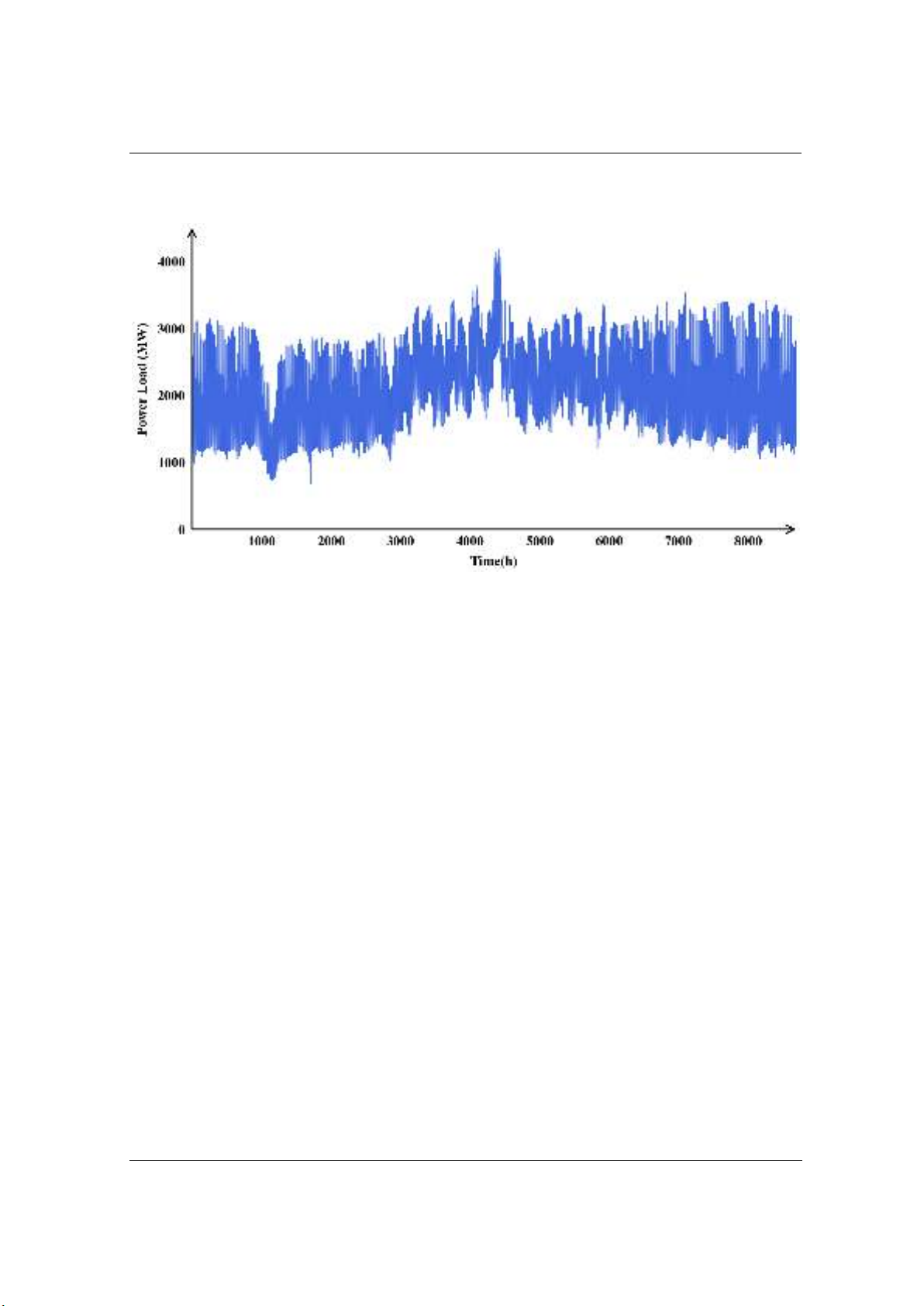
The data set utilized by the proposed and comparison models in this study is the recorded load
data of Hanoi in 2018. The data was collected from 1/1/2018 0:00 to 12/31/2018 23:00 with a
TNU Journal of Science and Technology
229(06): 220 - 229
http://jst.tnu.edu.vn 222 Email: jst@tnu.edu.vn
sample every 1 hour. Due to this sample interval, the number of data points were 8760 data point.
A visualization of the raw load data is presented in Figure 1. The load data was recorded in MW.
Figure 1. Hanoi load data in 2018
Outliers, which are data points significantly different from the rest of the dataset and can have
a substantial impact on model performance [10]. Similarly, the presence of missing values
represents a common issue that can disrupt analytical processes and model training if left
unresolved. Consequently, data preprocessing plays a pivotal role in ensuring the quality and
reliability of the data used for the models. In this paper, both of these issues were addressed by
using graph visualization techniques. Initially, a graphical representation was generated from the
original dataset to facilitate the evaluation process. Subsequently, this graphical representation
was scrutinized to identify outliers and missing values, thus facilitating further processing. Any
identified anomalies or missing data were subsequently corrected or eliminated from the dataset,
ensuring its suitability for subsequent model training endeavors.
Apart from outliers and missing values, it is noteworthy that many machine learning models
are sensitive to data scales, leading to the need for data scaling. In this paper, max-min
normalization and z-score standardization were used to carry out the scaling process. Max-min
normalization rescales the data values to a range between 0 and 1 while z-score standardization is
used to transform the values to be normally distributed with a mean of zero and a standard
deviation of one [11].
2.2. Extreme Learning Machine
Feed-forward neural networks, such as Convolutional Neural Networks (CNN) or Multilayer
Perceptron (MLP), have been utilized in various fields including image classification, natural
language processing, and speech recognition [12] - [14]. Extreme Learning machine is a learning
algorithm invented for the purpose of training Single-hidden-layer feedforward neural networks
(SFLNs). Different from traditional feed-forward neural networks where all parameters need to
be tuned, the input weight and biases of the hidden layer in ELM are randomly initialized [7].
Because of this, ELM has been known to perform exceptionally fast with good performance
when compared to traditional feed-forward neural networks models.
TNU Journal of Science and Technology
229(06): 220 - 229
http://jst.tnu.edu.vn 223 Email: jst@tnu.edu.vn
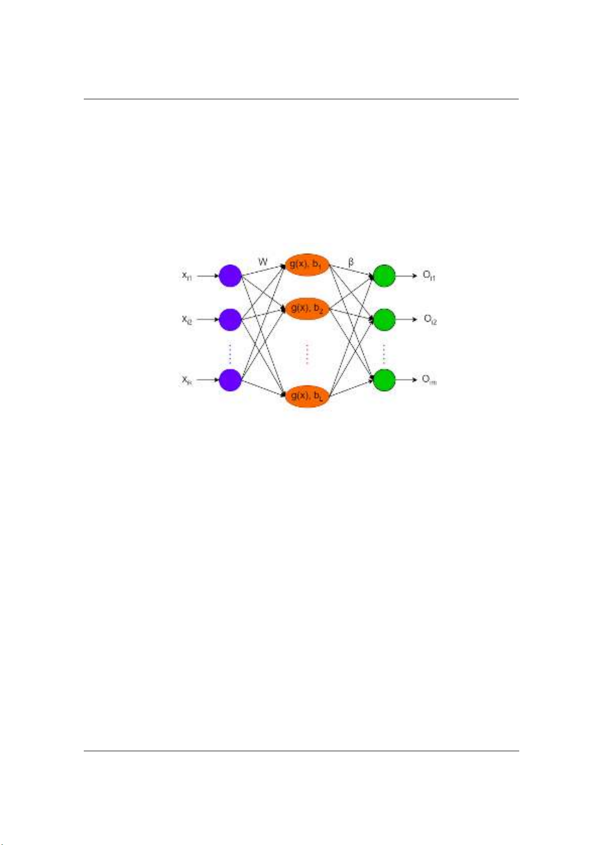
For N number of random training sets (𝑋𝑖,𝑌𝑖) where 𝐗𝐢=[𝑥𝑖1,𝑥𝑖2,…,𝑥𝑖k]⊤∈𝑅𝑘 is the model
input and 𝐘𝐢=[𝑦𝑖1,𝑦𝑖2,…,𝑦𝑖m]⊤∈𝑅𝑚 is the model output, L is the number of hidden nodes and
g(x) is the activation function, because the model output and expected output are equal in ELM
model calculation, the output function expression of the ELM can be expressed as :
𝑡ℎ𝑒 ∑
𝐿
𝑙=1 𝛽𝑙𝑔(𝑏𝑙+𝑊𝑙⋅𝑋𝑖)=𝑂𝑖=𝑌𝑖, 𝑖=1,…,𝑁
(1)
Where, 𝐖𝐥=[𝜔𝑙1,𝜔𝑙2,…,𝜔𝑙k]⊤ is the input weight matrix in between input to lth hidden
nodes, 𝛃𝐥=[𝛽𝑙,𝛽𝑙2,…,𝛽𝑙m]Tis the output weight matrix in between lth hidden nodes to the output
node. The output of ELM is considered as 𝑂𝑖. The specific structure of the model can be
described in Figure 2.
Figure 2. The structure of ELM
Eq. (1) can be described using Eq. (2)
𝐇𝛃=𝐘
(2)
In Eq. (2), 𝐇 is the hidden layer output matrix. The formulas for 𝐻,𝛽, and 𝑌 are shown in Eqs.
(3) and (4), respectively.
𝐇=[𝑔(𝑋1⋅𝑊1+𝑏1)⋯ 𝑔(𝑋1⋅𝑊𝐿+𝑏𝐿)
⋮ ⋱ ⋮
𝑔(𝑋𝑁⋅𝑊1+𝑏1)⋯ 𝑔(𝑋𝑁⋅𝑊𝐿+𝑏𝐿)]𝑁×𝐿
(3)
𝛃=[𝛽1𝑇
⋮
𝛽𝐿𝑇]𝐿×𝑚𝐘=[𝑌1𝑇
⋮
𝑌𝑁
𝑇]𝑁×𝑚
(4)
In the ELM model parameter training process, if 𝑊
‾𝑙,𝑏‾𝑙, and 𝛽‾𝑙 can make Eq. (5) hold:
𝐸=min𝑊,𝑏,β ∑𝑖=1
𝑁 (∑𝑙=1
𝐿 𝛽‾𝑙𝑔(𝑊
‾𝑙⋅𝑋𝑖+𝑏‾𝑙)−𝑌𝑖)2=minW,b,β∥𝐇𝛃−𝐘∥
(5)
Then 𝑊
‾𝑙,𝑏‾𝑙 and 𝛽‾𝑙 are the optimal ELM model parameters. In the ELM model, once the input
weight 𝑊 of the model and the hidden layer threshold 𝑏 are determined, the output matrix 𝐇 of
the hidden layer is uniquely determined. Under this condition, the ELM learning process can be
transformed into a linear system (6).
𝛃
‾=𝐇−𝟏𝐘
(6)
In Eq. (6), 𝐇−𝟏 is a generalized inverse matrix. It can be seen from the above discussion that the
ELM training process involves continuously seeking the optimal solution of the nonlinear system.
TNU Journal of Science and Technology
229(06): 220 - 229
http://jst.tnu.edu.vn 224 Email: jst@tnu.edu.vn
2.3. ELM modeling and forecasting process
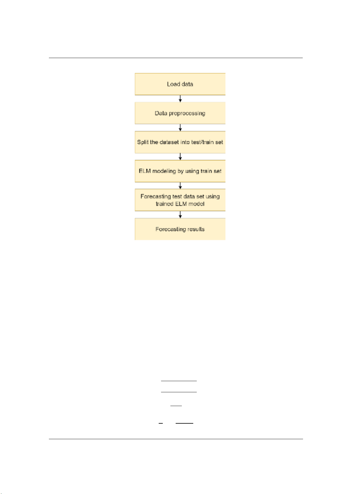
Figure 3. Flowchart of the forecasting process
Figure 3 illustrates the forecasting process through a flowchart. Initially, the load data is
acquired and subjected to preprocessing, employing techniques such as data cleaning or
normalization. Subsequently, the dataset was divided into a training set and test set with a
distribution ratio of 90/10. The training set was employed to train the proposed model, whereas
the test set was allocated to conduct the forecasting process. The forecasting results are obtained
upon the completion of the forecasting process.
The input data for the models comprised 48 historical data points extracted from the dataset
sampled at hourly intervals, including the data from time t to t-47. The output of the forecasting
models varies depending on the number of forecasting steps, including data at time t+1, t+2,..., t+
k where k is the number of forecasting steps. For instance, in single-step forecasting, the output
corresponds to t+1, while in 3-step forecasting, the output comprises the data at t+1, t+2, and t+3.
2.4. Error metrics
In this study, three error metrics were employed for the evaluation of the proposed model.
These metrics include the Root Mean Square Error (RMSE), normalized RMSE (n-RMSE), and
Mean Absolute Percentage Error (MAPE). The lower the value of these error metrics, the better
the forecasting result. RMSE, n-RMSE and MAPE are defined as follows:
𝑅𝑀𝑆𝐸=√∑(Oi−Ei)2
N
i=1 N
(7)
𝑁_𝑅𝑀𝑆𝐸=RMSE
O
× 100
(8)
𝑀𝐴𝑃𝐸=1
N ∑|𝑂𝑖−E𝑖
𝑂𝑖|
𝑁
𝑖=1
(9)


![Bộ tài liệu Đào tạo nhân viên chăm sóc khách hàng tại đơn vị phân phối và bán lẻ điện [Chuẩn nhất]](https://cdn.tailieu.vn/images/document/thumbnail/2025/20251001/kimphuong1001/135x160/3921759294552.jpg)


![Thiết kế tụ điện và đi dây [chuẩn nhất]](https://cdn.tailieu.vn/images/document/thumbnail/2018/20180612/truonganhshun/135x160/9041528775303.jpg)


![Chương trình đào tạo cơ bản Năng lượng điện mặt trời mái nhà [mới nhất]](https://cdn.tailieu.vn/images/document/thumbnail/2026/20260126/cristianoronaldo02/135x160/21211769418986.jpg)

![Chương trình đào tạo cơ bản Năng lượng gió [Tối ưu SEO]](https://cdn.tailieu.vn/images/document/thumbnail/2026/20260126/cristianoronaldo02/135x160/53881769418987.jpg)


