Copyright © IFAC
12th
Triennial World Congress.
Sydney. Australia. 1993
AUTOMATIC
TUNING OF
DECENTRALIZED
PID
CONTROLLERS
FOR TITO
PROCESSES
Z .
.I.
Paltnor,
Y.
Halcvi
and
N.
Krasncy
Fuculty
of
Mccizani"al
En}!.in('('fin}!..
T('cizllion . I/aifel 3200(]. Israel
Abstract
The
paper presents a new automatic tuning algorithm for Decentralized PID Control
for
two
inputs -
two
outputs (TITO) plants.
The
tuning procedure. which is an extension
of
the
Ziegler-Nichols method requires identification
of
a critical point consisting
of
critical gains
of
the various loops and a critical frequency. Unlike
SISO
plants there are infinitely many such
points and
knowledge
of
the desired one is essential to the tuning procedure.
The
auto-tuner
identifies
the
desired
critical point with no apriori information
of
the process. During the
identifiction phase all controllers are replaced by relays. thus generating limit
cycles
with the
same
period in both loops. It
is
shown that this limit cycle corresponds to a single critical point
of
the process. By varying the relays parameters different critical point can be determined.
The
auto-tuner
contains
a
procedure
which
converges
rapidly to the desired critical point while
maintaining the amplitudes
of
the process variables within prespecified ranges.
The
steady-state
process
gains. which are required for the appropriate
choice
of
the desired critical point, are
determined in closed-loop fashion simultaneously with the identification
of
the critical points. It
is shown that the proposed auto-tuner
is
more efficient and reliable than a recently published
algorithm
and
works
well also
in
cases
where the laller algorithm fails to
converge
and even
destabilizes the system.
Keywords: Decentralized Control; Automatic Tuning; Interactions;
PlO
Control.
I.
INTRODUCTION
Decentralized
PlO
control is
one
of
the most
common
control
schemes
for interacting multiple-input multiple-output (M1MO)
plants in the
chemical
and process industries.
The
main reason
for
this is its
relatively
simple
structure
which is
easy
to
understand and
to
implement.
The
number
of
tuning parameters
IS
3n where n
IS
the
number
of
inputs and outputs while in full
matrix
PlO
control
there
are 3n2
parameters.
Even
for
moderate
size
systems
this is a significant reduction.
In
case
of
actuator
or
sensor
failure,it
is
relatively
easy
to
stabilize
manually
be~ause
only
one
loop is directly affected by the
faIlure.
Desplle
llS
Simple structure. decentralized PID control
has a long record
of
satisfactory perfonnance.
We
turn
now
to the
problem
of
tuning these controllers. It is
assumed
throughout
this
paper
that an analytic model
of
the
process
is not available and the tuning procedure is based on
expenmental
data. Even for single-input single-output (SISO)
systems
the tuning
of
a
PlO
controller is not an easy task.
The
most
common
design procedure is the Ziegler-Nichols method
(Zlegler
and
Nlchols,
1942).
The
fundamental
step
in that
method
is the
identification
of
the critical gain and critical
frequency
of
the plant. that together are called the critical point.
Based
on
these values, the controller gain and the integral and
derivative
coefficients
are calculated.
In
MIMO
svstem
the
tuning
problem
is
many
times
more
complicated
due
to the
interactions
between
loops. A
change
of
a single
parameter
affects. in
general,
all
other
loops as well in a way which is
hard to predict.
Only
a limited number
of
works addressed the
tuning
of
decentralized
PID controllers. Marino-Gallarraga
et
al.
(1987)
presented
a
design
method
which
combines
information
regarding
the
MIMO
system
performance
and
SISO
properties
of
each
loop.
The
method
in
(Niederlinski,
1971) is a
more
natural extension
of
the Ziegler-Nichols tuning
procedure
to the
MIMO
case
.
It
is based on
replacing
the
controllers
by
gains
and
identification
of
a
critical
point
~onsisting
of
n scalar critical gains and the critical frequency.
rhe
main
departure
fomlthe
SISO
case is that
MIMO
systems
lave
infinitely
many
critical points.
The
collection
of
these
'oims
define
a hypersurface in the gains space which is called
he
stability
limits.
Consequently
one
has to
prespecify
the
lesired
critical
point,
e.g.
equal
loop
gains.
Once
the
.Jarameters
of
the critical point are detcmlined the controllers are
tuned in a similar fashion to the classical Ziegler-Nichols rules.
The
direct application
of
the Ziegler-Nichols mcthod has
some
shortcomings.
The
procedure
involves
trial
and
error
experiments
to
identify
the
critical
point.
During
these
experiments
the system might be unstable for a period
of
time.
which is risky. When the critical point
is
identified. there
is
no
control
over
the
amplitude
of
oscillations
of
the
process
73
·
nriablt:.
In
addition the
procedure
requires
an
experienced
operator
and is time consuming.
The
same problems exist for
thc
MIMO
case
and
are
even
more
severe.
Astriim
and
Ilagglund
(1984 and 1988) suggested the use
of
a relay in the
identification phase for a
SISO
system. Instead
of
a system on
the verge
of
instability the critical point is identified from a
stable limit cycle.
This
is also very convenient for auto-tuning
where by selling a tuning mode the
PlO
controller is replaced
by a relay, the critical point is identified and the parameters are
updated.
(Zgorzelski
. 1988) and
(Zgorzelski
et
aI., 1990)
extended
that idea to the
MIMO
case.
In
their approach
one
controller
is
replaced
by
a
relay
while
the
others
by
P
controllers
whose
values
are
adjusted
in
each
of
the
experiments until the desired critical point
is
obtained.
In
this
paper
we suggest a new algorithm for auto-tuning
of
decentralized
PlO
controllers for two-input two-output (TITO)
systems.
The
main departure from the method
of
(Zgorzelski et
aI., 1990)
is
that the controllers
in
all the loops are replaced by
relays. Each
such
experiment
identifies a critical point. By
varying the magnlludes
of
the relays the identified critical point
moves
along
the stability limits.
The
algorithm
changes
the
magnuudes
of
the relays such that convergence to the desired
critical point is obtained within a small number
of
experiments.
Funhermore,
the steady state gains needed for the definition
of
the critical point, are identified simultaneously with the critical
gains and frequency and
do
not require a separate experiment.
The
material
is
organized
as follows:
In
section 2 a
short
review
of
the auto-llIncr for
SISO
system is given. Section 3
discusses
the
manual
lUning procedure for
TITO
system
and
sec lIon 4 describes the
suggested
auto-tuner.
The
results are
summarized and discussed in section
5.
2.
AUTO-TUNING
OF
PID
CONTROLLER
FOR
SISO
SYSTEMS
We start by a
shon
review
of
the auto-tuner for
SISO
systems.
The
problem
is
as
follows:
Given
a
stable
but
otherwise
unknown plant pes) find a selling
of
the PID controller
C(s) =
K(!
+
R/s
+ Os)
(2.1)
that gives satisfactory performance. (In practice the derivative
part contains a filter with a time constant which is proportional
to 0 but
much
smaller).
The
most
common
and
useful
approach to the problem is the Ziegler-Nichols (1942) design
method.
The
first step in this
method
is to
replace
the
PID
controller by a proportional controller and gradually increase its
gain until the
system
reaches
a state
of
neutral stability. i.e.

oscillation with constant amplitude. The gain which achieves
that is called the critical gain
Kcr
and the frequency
of
oscillations, which is calculated from their time period,
is
called
the critical frequency w
cr
. The parameters
K,
Rand
Dare
then given as
K = aKcr. D =
y/w
cr
(2.2)
where
a,
~
and y are
constants
and there are several
suggestions for their exact values. [f a Nyquist plot
of
the plant
is available then
Kcr
and
W<~
can be calculated out
of
it.
At W
=
Wcr
the plot crosses the negative real axis and the intersection
point is -I/Kcr.
The above mentioned experimental procedure for detennining
Kcr
and
W<~
has some shortcomings. During the trial and error
phase the gain might be set too high thus giving rise to a
temporary state
of
instability which is risky. Even
if
this is
avoided
there is no control
over
the
amplitude
of
the
oscillation.
That
may lead to unacceptable response
or
to
distortion
of
the signals, thus also incorrect critical gain and
frequency, due to saturation.
To
circumvent those difficulties
it
was suggested (Astrom and Hagglund,
19B4
and 198B) to
use relays
in
the identification process and to calculate
Kcr
and
Wcr from the stable limit cycles that are reached. Under the
standard
assumptions
of
the
describing
function
Kcr
is
calculated from
4M
Kcr=-
na (2.3)
where M and a are the relay and the limit cycle amplitudes
respectively. w cr is calculated as before from the time period
of
the response. [n addition to the superior robustness
of
this
procedure, the amplitude a can be adjusted
by
appropriate
selection
of
M. [n case
of
noisy measurement the ideal relays
may be replaced
by
a relay with hysteresis.
[n
such cases there
is a trade-of between the insensitivity to noise, which requires
larger hysteresis and the accuracy
of
the fonnula for Kcr that
corresponds to zero hysteresis.
An advantage
of
the relay-based method is that it is suitable for
auto-tuning. When the auto-tuner is set to the tuning mode the
controller is replaced
by
a relay and the experiment begins. The
limit
cycle
time period is
detennined
by
measuring
time
between zero crossings and its amplitude from peak to peak
values.
These
values are then used to update the controller
parameters.
3.
TUNING
PROCEDURE
FOR
TITO
SYSTEMS
Stability Limits
ofT/TO
Systems. Consider now the system in
Fig. I which is the basic scheme
of
decentralized control. The
first step in extending the results
of
the previous section to
T[TO (or
in
general to MIMO) systems
is
to
define the stability
limits.
[n
S[SO systems there is only a finite number
of
critical
gains that brings the system to the verge
of
instability. [n most
cases there is only one such gain. [n the system
in
Fig. I, on
the
other
hand, there are infinitely many gains (k l, k2) that,
when replacing Cl (s) and C2
(S),
lead to neutral stability, i.e.
poles on the imaginary axis. The collection
of
all these gains is
called the stability limits
of
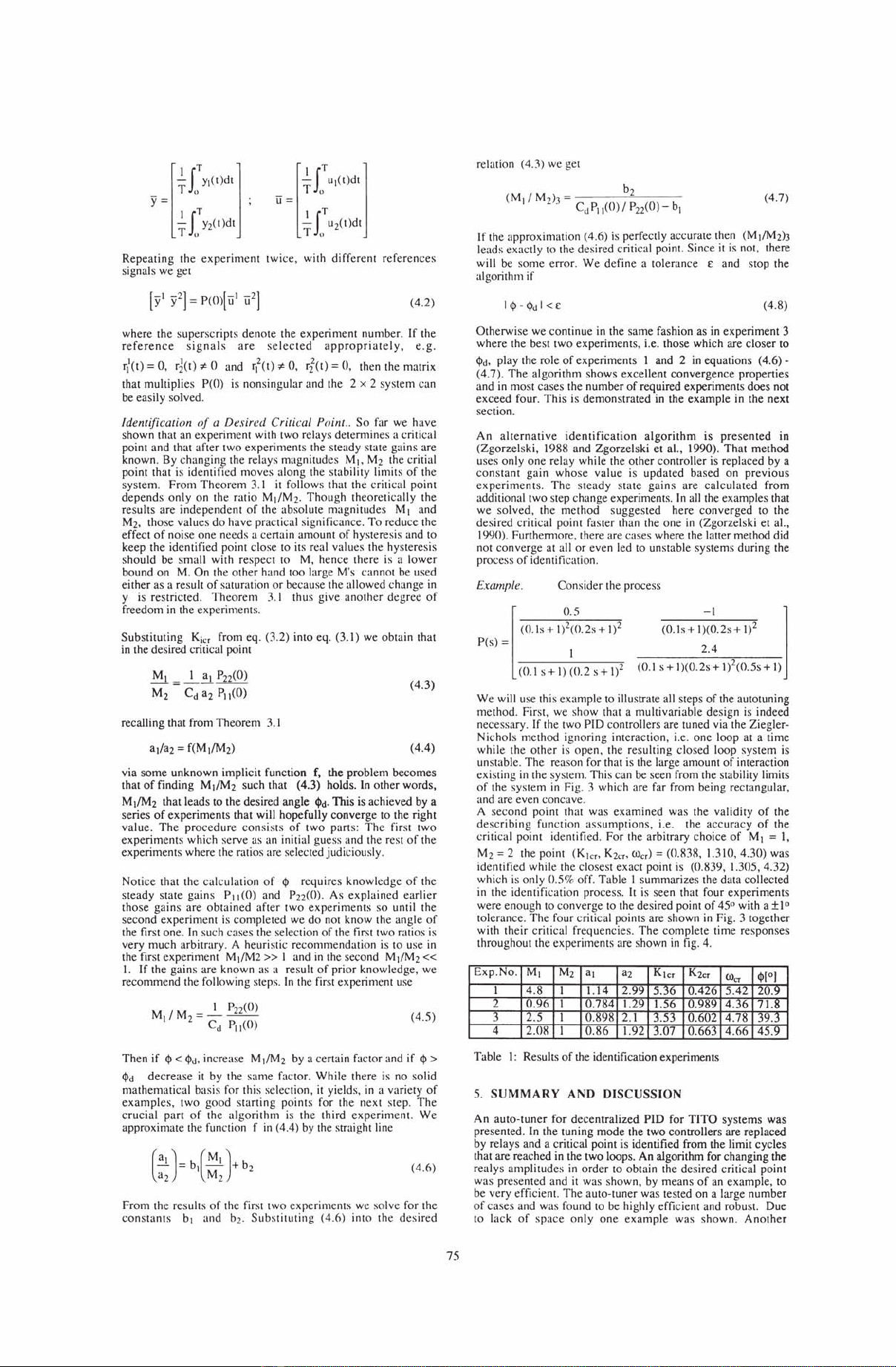
the system. Three typical cases
of
the stability limit are shown
in
Fig. 2. Since the significant
parameter perfonnance is the loop gain, the axes are kjPjj(O).
Each point on the curves corresponds to a pair
of
gains
(k
1cr
,
k2cr)
and a critical frequency w
cr
.
[n
the sequel we refer
to
it
as
a critical point. The points on the axes represent the situation
where one loop is open (ki = 0) hence the
other
gain is the
S[SO critical gain
of
the other loop. [f the system does not have
full interaction, i.e. either P
12
(s)
or
P21(S)
or
both are zero,
the stability limits take the rectangular fonn.
[n
that case the two
critical gains are independent
of
each
other
and the system
becomes unstable when either one
of
the gains exceeds its
S[SO critical value.
The
other two curves represent systems
with interaction. The deviation from the rectangular shape may
be regarded as a (rather crude) measure
of
interaction.
On
the
basis
of
a (for the time being arbitrary) critical point one can
tune the P[D controllers either via the Ziegler-Nichols method
in eq. (2.2) or its modifications
in
(Niederlinski, 1971).
Clearly, different critical points lead to different controllers,
hence different perfonnance. lt is well known that a larger loop
74
gain results
in
a tighter control.
Thus
if
one
loop is
more
important than the other we would like
it
to have a larger loop
gain which in interacting systems usually means that the
other
loop will have lower gain. The relative importance
of
the loops
corresponding to a particular point can therefore be described
by
the ratio
(3.1 )
where
q,
is the angle
of
the line connecting the critical point to
the origin.
For
a given desired ratio
Cd
and assuming that the
steady state gains P11(0) and P
22
(O)
are known,
one
can
increase the two gains simultaneously while keeping the ratio
between them. However this procedure suffers from the same
shortcomings as its SISO counterpart, as discussed in section
2.
The
motivation for the use
of
relays is therefore also the
same.
Multivariable Limit Cycles. Consider the system in Fig. I but
with the controllers replaced by relays having magnitudes Mt
and
M2.
Under most circumstances stable limit cycles in both
loops are reached. Those limit cycles have the following
properties: (i)
Common
time period T (unless the plant is
decoupled) (ii) Different amplitudes, denoted by al and
a2
(iii)
Time
shifts
between
the cycles, i.e. the loops are
asynchronous.
An important result which is utilized
in
the design procedure
in
the next section is as follows.
Theorem 1 1 (Krasne}',
19911:
Consider the system in Fig.
\.
but with relays. All pairs
(M(.
M2) such that Mt
/M2
=
constant lead to limit cycles with the same time period T, the
same time shift y and the same ratio
of
amplitudes
ada2.
If
the relays contain hysteresis b" the above mentioned results
hold
if
the proportions bt/M t and
b2fM2
are retained.
Remark:
Theorem
3.1
is a special case
of
a
more
general
result for
M[MO
systems (Palmor et aI., 1992).
In
(Krasney,
1991) it is
shown
that when the
standard
describing
function
assumptions
are
met,
a
good
approximation
of
a critical point is
4M
Kicr =
--'
nai
wcr=2nlT
i = 1,2 (3.2)
(3.2)
Hence by using two relays a critical point is identified. Notice
that
Theorem
3.1
implies that all pairs (M
I,
M2) such that
M
t/M2
is
constant
correspond
to
one
critical point.
The
problem that remains is the identification
of
a desired critical
point, i.e. a given ratio C.
4.
THE
AUTO-TUNER
Determination
of
Steady State Gains. As was mentioned earlier
the important factor is the relative magnitude
of
the loop-gains
and not that
of
the
controller
gains as such.
That
requires
knowledge
of
the steady state gains
of
the process
Pji(O)
. Since
the underlying assumption
of
this paper is that no analytical
model
of
the process is available we have to identify those
gains
experimentally.
The
most
straightforward
way
of
calculating the gains is to change
Uj
by a constant t.Uj, wait
for
convergence
and then
Pij(O)
= t.yJt.Uj.
This
method
is
time consuming and also raises some practical questions such
as how to define convergence etc. A faster
and
more elegant
approach is to identify the gains from the response to a finite
pulse. However, that method also requires a separate dedicated
experiment. Since we wish to make
as
few
experiments
as
possible we use the relays setup
to
identify the steady state
gains
simultaneously
with identification
of
critical
points.
Consider
the system
in
fig. I with relays and with rt (t), r2(t)
which are not both zero mean. Then the error signals ei and
the controls
Uj
are also nonzero mean. From a
DC
balance,
or
in mathematical
tenns
comparing
the constant
terms
of
the
Fourier series, we get
y=
P(O)u
(4.1 )
where
If
-YI(I)dt
T
()
If
-uI(t)dt
T
()
y=
u=
If
-Y2(t)dt
T
()
If
-u2(t)dt
T
()
Repeating
the
experiment
twice,
with
different
references
signals
we
get
(4.2)
where the
superscripts
denote
the
experiment
number.
If
the
reference
signals
are
selected
appropriately,
e.g.
ri(t)
= 0,
d(I)"#
0
and
r?(I)"# 0,
ri(I)
= 0, then the matrix
that
multiplies
PtO) is
nonsingular
and
the 2 x 2
system
can
be
easily
solved.
IdenrificQlion
of
a
Desired
Critical Point
..
So
far
we
have
shown that an
experiment
with two relays
determines
a critical
point
and
that
after
two
experiments
the
steady
state
gains
are
known. By
changing
the relays
magnitudes
M1,
M2
the critial
point that is identified
moves
along
the stability limits
of
the
system.
From
Theorem
3.1 it follows that the
critical
point
depends
only
on
the
ratio
MI/M2.
Though
theoretically
the
results
are
independent
of
the
absolute
magnitudes
M I
and
Ml,
those
values
do
have
practical significance.
To
reduce
the
effect
of
noise
one
needs
a certain
amount
of
hysteresis
and
to
keep
the identified point
close
to its real values the hysteresis
should
be
small
with
respect
to M,
hence
there is a
lower
bound
on M.
On
the
other
hand
too
large M's
cannot
be used
either
as a result
of
saturation
or
because the allowed
change
in
y is
restricted.
Theorem
3.1 thus
give
another
degree
of
freedom in the experiments.
Substituting
Kicr
from
eq. (3.2) into eg. (3.1) we
obtain
that
in the desired critical point
~=~~P22(O)
M2 Cd
a2
PII(O)
recalling that from
Theorem
3.1
(4.
3)
(4.4)
via
some
unknown
implicit
function f, the
problem
becomes
that
of
finding MJlM2 such that (4.3) holds.
In
other
words,
MI!M2 that
leads
to the desired angle
ci>d-
This
is achieved by a
series
of
experiments
that will
hopefully
converge
to the
right
value
.
The
procedure
consists
of
two
parts:
The
first
two
experiments
which
serve
as an initial guess
and
the rest
of
the
experiments
where the ratios are selected judiciously.
Notice
that the
calculation
of
<I>
requires
knowledge
of
the
steady
state
gains
PII
(0)
and P12(0).
As
explained
earlier
those
gains
are
obtained
after
two
experiments
so
until the
second
experiment
is
completed
we
do
not
know
the
angle
of
the first
one
.
In
such
cases
the selection
of
the first
two
ratios is
very
much
arbitrary. A heuristic
recommendation
is
to
use
in
the first
experiment
MI!M2»
I and in the second
MI!Ml«
I.
If
the
gains
are
known
as a result
of
prior
knowledge
,
we
recommend
the following steps.
In
the first experiment use
(4.5)
Then
if
<I>
<
<l>d,
increase M t/M2 by a certain factor
and
if
<I>
>
<l>d
decrease
it
by
the
same
factor.
While
there
is no solid
mathematical
basis
for this selection,
it
yields, in a variety
of
examples
,
two
good
starting
points
for the next step.
The
crucial
part
of
the
algorithm
is the
third
experiment.
We
approximate
the function f in (4.4) by the straight line
(4.6)
From
the
results
of
the first
two
experiments
we
solve for the
constants
bl
and
bl .
Substituting
(4.6)
into
the
desir
ed
75
relation (4.3)
we
get
(4.7)
If
the
approximation
(4.6)
is
perfectly accurate then
(MI!M2h
leads
exactly
to
the desired critical point.
Since
it is not, there
will be
some
error.
We
define
a
tolerance
E
and
stop the
algorithm
if
(4.8)
Otherwise
we
continue
in the
same
fashion as in
experiment
3
where
the best
two
experiments,
i.e. those which are
closer
to
<l>d,
play the role
of
experiments
I and 2 in
equations
(4.6)-
(4.7).
The
algorithm
shows
excellent
convergence
properties
and
in
most
cases
the
number
of
required
experiments
does
not
exceed
four.
This
is
demonstrated
in the
example
in the
next
section.
An
alternative
identification
algorithm
is
presented
in
(Zgorzelski,
1988
and
Zgorzelski
et
aI., 1990).
That
method
uses
only
one
relay
while
the
other
controller
is replaced by a
constant
gain
whose
value
is
updated
based
on
previous
experiments
.
The
steady
state
gains
are
calculated
from
additional
two
step
change
experiments.
In
all the examples that
we
solved,
the
method
suggested
here
converged
to the
desired
critical point faster than the
one
in
(Zgorzelski
et
aI.,
1990). FurthemlOre, there are
cases
where the latter method did
not
converge
at all
or
even led to unstable
systems
during the
process
of
identification.
Example.
Consider
the process
-I
1
(O.ls + 1)(0.2s +
1)2
2.4
0.5
pes) =
(0 I
s+
1)(0.2s+
1)2(0.5s+
I)
(0.1
s+
I)
(0.2
s+
1)2
We
will use this
example
to illustrate all steps
of
the autotuning
method
. First, we
show
that a
multivariable
design
is indeed
necessary. If the
two
PID controllers
are
tuned via the Ziegler-
Nichols
method
ignoring
interaction, i.e.
one
loop
at a time
while
the
other
is
open,
the
resulting
closed
loop
system
is
unstable.
The
reason for that is the large
amount
of
interaction
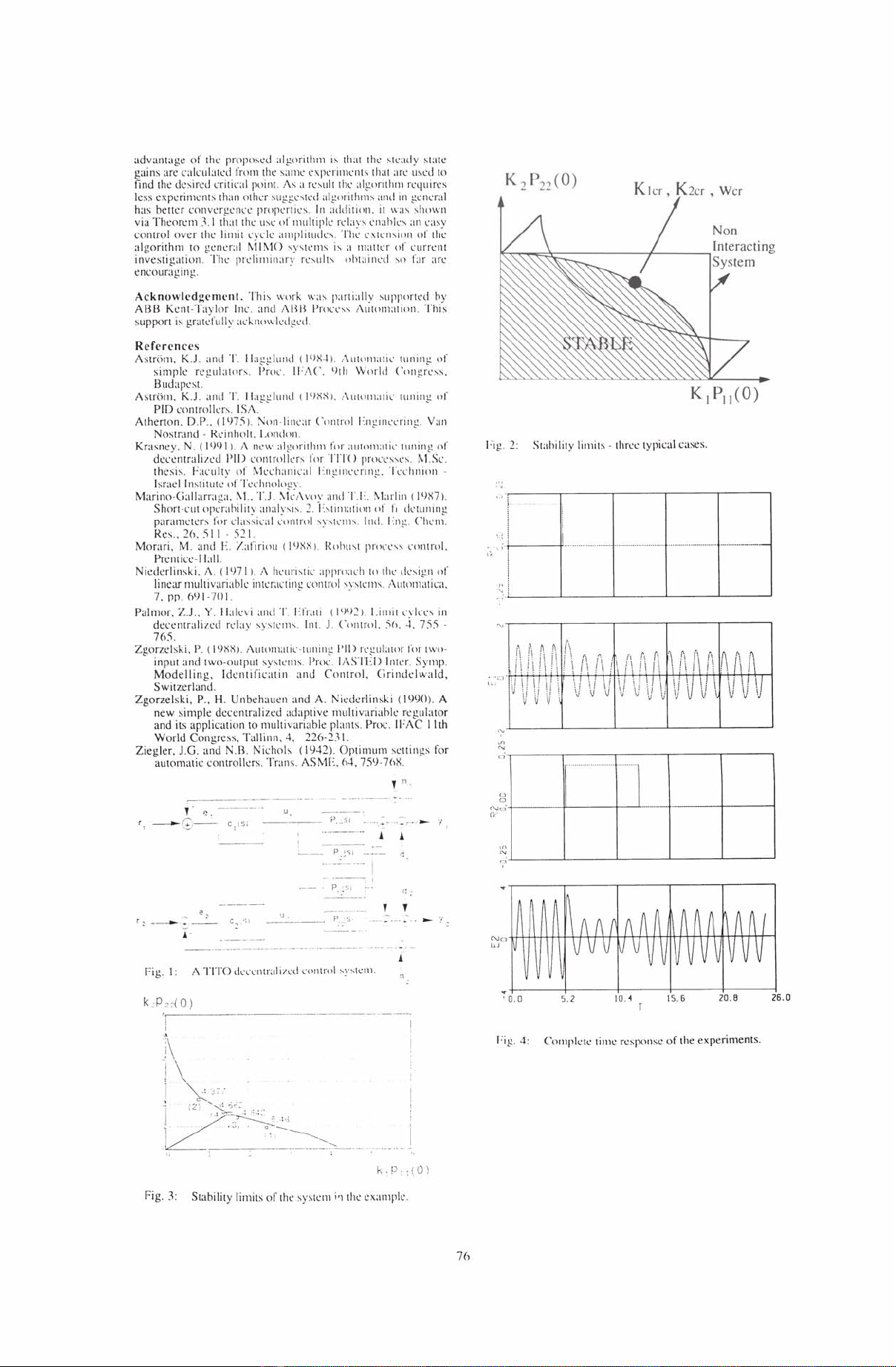
existing in the system.
This
can
be seen from the stability limits
of
the
system
in Fig. 3 which are far from being rectangular,
and are even concave.
A
second
point that
was
examined
was
the validity
of
the
describing
function
assumptions
, i.e. the
accuracy
of
the
critical point identified.
For
the arbitrary
choice
of
MI =
I,
M2 = 2 the point (K lcr,
Kl
cr
, w
cr
) = (0.R38,
1.310,4.30)
was
identified
while
the closest
exact
point is (0.
839
,
1.305,4.32)
which is
only
0.5% off.
Table
I
summarizes
the data collected
in the
identification
process. It is seen that four
experiments
were
enough
to
converge
to the desired point
of
45" with a ±Io
tolerance
.
The
four critical points are shown in Fig. 3
together
with
their
critical
frequencies
.
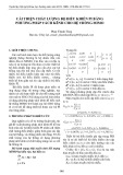
The
complete
time
responses
throughout the
experiments
are shown
in
fig. 4.
Exp.No.
MI
M2
al
a2
Klcr
K2cr
wc,.
<1>[0)
I
4.8
I
1.14
2.99
5.
36
0.426
5.42
20.9
2
0.96
I
0.784
1.29
1.56
0.989
4.36
71.8
3
2.5
I 0.R98 2.1
.3
.
53
0.602
4.78
39
.3
4 2.0R I 0.
86
1.92
3.07
0.663
4.66
45.9
Table I : Results
of
the identification experiments
5.
SUMMARY
AND
DISCUSSION
An
auto-tuner
for
decentralized
PlO
for
TITO
systems
was
presented. In the
tuning
mode
the
two
controllers
are
replaced
by relays
and
a critical point is identified from the limit
cycles
that are reached in the
two
loops.
An
algorithm for changing the
realys
amplitudes
in
order
to obtain the desired critical point
was
presented
and
it
was
shown,
by
means
of
an
example,
to
be very efficient.
The
auto-tuner
was tested on a large
number
of
cases
and was found to be highly efficient and robust.
Due
to
lack
of
space
only
one
example
was
shown
.
Another
advantage
or
th
e:
[lro[lme:d ;d
gor
itlull is that t
he
"e;
ld
y
"ate
ga
in
s arc calc
ul
at
ed
fwm
the same
L"
p<:rin1ent
s
th
;
1I
ar
e:
med to
fi
nd
th
e desired
cr
i
ti
c;
d point. As a
r<:>
ult the
al
gorithm requ ires
le
ss
e
xpaim
en
ts
th
an o
th
er suggcsted algllrithms a
nd
in
gcnc
ra
l
has better convergcncc prope
rt
ics. In ;Iddit ion. it
\\,;IS
shllwn
v
ia
Theorcm 3.1
th
;
1I
t
he:
u"
of multiple rL'
Ia
\,s
en;d1ks an casy
control over the lim
it
c)'L'
1c
;Im
plitud e.s. Thc
L'\l
Cn
si
lln
of
th
e
al
gor
ithm to
ge:
ncral M I MO systL
'm
s is ;1 matt
er
Ilf current
investigation. T
hc
prelin
1ina
r
\'
rc
sults o
bt
aincd
\(
'
fa
r a
rc
encourag
in
g.
Ac
knu
wlcdgc nll'lIt. This work
w;"
partially supported hy
ABB
Kcnt-
Ta
vl
or
Inc and AIlIl I'ro
CL'SS
Au
tll
m;
lIi
on. T
hi
s
s
U[lp
o
rt
is grat
:r
u
lly
ack nowledgcd.
Referen
ces
Astr(im. K.J. a
nd
T.
lI
a~~lun
d
(I')
X-l).
,\uto1l1
;lI
ic tunin!.:
of
sim[llc r
q.!
ul
;
lI
or
s.
I
)
~oc
II'AC.
')
Ih World ('Ilngr'css.
Budapes
t.
As
tr
om.
KJ
. and T.
lI
a
~~lun
d
( I
')XX
I.
,\ ul
om
al
iL
'
l
u
ni
n~
of
PID controlle
rs.
I
SA
."
,
Atherton, D.P
..
(1<)
75
).
N
on
-
lin
ear Cllnlrol
Ln
~
in
L
·
erin
~
.
Van
Noslrand -
Rci
nholl. London . "
Krasnev.
N.
( I')l) I
).
A new
a
l
~or
il
h
m
fill'
a
UI,"1
1;
lI
i
L'
tunin
~
of
dcc
~
n
tr
a
li
ze
d
I'ID
co
ntrol
Ins
f
or
TIH)
pro
C·c
ss
L·
S.
r-.(Sl'.
thesi
s.
Facu
lt
\'
of Mcchanical
L
n~inL·L'ri
n
~.
T
L'L
'hnion -
Israc
ll
n
st
ilu
te'
of
T
ec
hn
ol
o
~
\
'
' ,
Marino-
Ciall
a
rr
;lga.
,,
1..
TJ .
\-I
L:
'
'''
o\,
an
d
TY
.
r-.
brl
in (
1')
X7).
Short-C
UI
opc-rahilily analys
is.
2.
Lslim;llillnllf f,
dC
lullin g
[laramcters f
or
classic
'a
l control sys
IL·n1s.
I
nd
. Lng.
('h
em.
Res
..
26.
:;
I I
52
1.
Morari, M. alld E. I .afiriou ( I
')
XX
I.
Rohusl
IlI"ll
eL
'ss clllltml.
Pren
ti
ce-Ila
ll
.
Niederlinsk
i.
A. (I '
)7
I
).
A h
L'u
r
"l
iL' apprll;
IL'i
1 I
II
Ihe
'ks
ig
ll
of
linear multiv
ari
ablc
illlcrac
·
t
i
n ~
contwl
"'ste
ms. Autom
ati
ca,
7.
pp
.
6'J1
-
71l
1 ' -
Palmor.
ZJ
..
Y. I
ble\
'i a
lld
'I' I
fLll
i ( I
'
)l)
~)
.
Limil l'\'
iL'e
s in
decenlralized
re
la
y sy
SlL·nl\
. l
il
t.
J. Cllll lro l. )
1,
. -
i.
75)
-
765.
Zgorzelsk
i.
P. (
Il)
XX).
AU
lomatic-
tu
ni
ng
I' ll)
rL
'gu
la
lllr for two-
input and two-output systcn
1s
.
I'w
c.
lASTED In
te
r.
Symp.
Mode
ll
in
g, I
dcn
ti
fi
cati n
and
Contr
ol, Cirindclwald,
Switzerland.
Zg
orzelski, P
..
H. Unbe hauen and A. Nicderlinski (
1<)<)Il
).
A
new simple decentralized ada[lt
iv
e mu
lt
ivariahlc
re
gu
la
t
or
and i
ts
applicat
io
n to multi variable rlant
s.
PW
l'.
II
''AC I I th
World Cong
re
ss. Ta
ll
in
n. 4, 226-
231
Ziegler, J.G. and
N.
B. Nichols (
19
42).
Ortim
um scttings
fo
r
automatic
co
ntroller
s.
Trans. ASME.
0-1
. 7 5
<)
-7 (
,'1',
.
, . 0
r
~
~:--.
C;
,
Si
e _
(:
~
...
---
r
c...,
,'
;)
u.
P
.,5)
~__
P
,
.
~"il
__
~_
--~.-
--- i
-
---,
p
..
~;i
r"
'
----
--
Fi
g.
I:
A 1'I
TO
dL'
L'c
lllrali
/c
d
L',,,lIJ'll
1 system.
, n
,
n .
Fig. 3: Sta
bi
l
it
y limits of t
he
system ;
'1
th
e examp
le
.
-
.,
76
K
ler,
K2cr ,
Wcr
Non
Fig. 2: Stability limi
ts
- three typical cases.
.'
~--
-,--
---.--
--,---
--.----.
,
;.
1-
--
--1
..
......
.........
......
.....................
..
....
....
.........
.. ..
"
'
L-
______
L-
____
~
__
____
~
______
-L
______
~
!\'\
~~
1\
(, r' \
~\
{\
j\
fd\
/1
; \
rl
!'\
.
1\
il!1
1\
1\
! 1 1\ ! 1
111\
1\
1\
II !\ !
1\
, iJ
I!
U
tI
\
I:
ij
. j
\1
\1
\1
\
\1
V
11
\
le
i
\!
\}
iJ
\i
11
i V i
~
V V V : V "
\;
V J
\i
\1
,n
~
T""-------r
-------,r_------,-------
-r-------,
u
o
~)t
:.
i
>--
--
--
'"
"
-
....
· 1
""
L
______
....L
__
____
....JL.
____
__
..L
______
....L
______
--'
No
-U-I+-I+-I+
++
-I--i
4-4+1-++-t+
I+
ffi-+-I-+l+hl-t++-I
+,H
"j
, 0. 0 5. 2
la
.
~
15. 6 20.8
26
. 0
Fig. 4: Complete time
re
sponse
of
the experiment
s.


![Giáo trình Thực hành Truyền động điện Trường Đại học Bà Rịa - Vũng Tàu [Mới nhất]](https://cdn.tailieu.vn/images/document/thumbnail/2026/20260310/hoaphuong0906/135x160/11121773283865.jpg)
![Giáo trình Thực hành SCADA Trường Đại học Bà Rịa - Vũng Tàu [Mới nhất]](https://cdn.tailieu.vn/images/document/thumbnail/2026/20260310/hoaphuong0906/135x160/94061773283866.jpg)
![Tài liệu học tập La bàn từ [mô tả/định tính]](https://cdn.tailieu.vn/images/document/thumbnail/2026/20260310/hoaphuong0906/135x160/25191773287376.jpg)

![Tài liệu học tập Thiết kế hệ thống nhúng [mới nhất, đầy đủ]](https://cdn.tailieu.vn/images/document/thumbnail/2026/20260305/hoatulip2026/135x160/37051773135929.jpg)


![Giáo trình Điều khiển khí nén thuỷ lực Phần 2: [Mô tả/Chủ đề cụ thể của phần 2]](https://cdn.tailieu.vn/images/document/thumbnail/2026/20260302/camtucau2026/135x160/11911772768225.jpg)
![Giáo trình Điều khiển khí nén thuỷ lực Phần 1: [Mô tả/Định tính thêm nếu cần]](https://cdn.tailieu.vn/images/document/thumbnail/2026/20260302/camtucau2026/135x160/51511772768225.jpg)
![Giáo trình Điều khiển số Phần 2: [Thêm từ khóa mô tả nội dung chương trình]](https://cdn.tailieu.vn/images/document/thumbnail/2026/20260302/camtucau2026/135x160/37201772766913.jpg)
