
REVIEW PAPER
A Review on PID Control System Simulation of the Active
Suspension System of a Quarter Car Model While Hitting Road
Bumps
Babak Shafiei
1
Received: 1 August 2021 / Accepted: 20 January 2022 / Published online: 21 February 2022
ÓThe Institution of Engineers (India) 2022
Abstract In recent years, car industry experts and
designers have given more attention to ensuring the safety
and comfort of the car and its passengers while traveling on
harsh road surfaces. This paper defines a simulation
approach for a quarter vehicle model with an active sus-
pension system using the SIMULINK environment in
MATLAB software. The first aim is to implement the
correct control system for an active suspension system of a
vehicle and a take closer look at the hydraulic cylinder and
servo valve concept details and its closed-loop control
system. And the second aim is to gain both ride comfort
and reliable road-holding by correctly tunning the PID
parameters for an active suspension system to reduce the
vehicle body displacement and acceleration. Furthermore,
the hydraulic pressure, hydraulic force, and total trans-
mitted force to the vehicle body are compared for active
and passive suspension systems when the car hits contin-
uous sinusoidal and random irregular bumps. The control
system is tuned via a PID controller using the Ziegler–
Nichols method via the Control System Designer app to
achieve the desired comfort traveling of passengers and
reliable ride-holding of the car. For an active suspension
system, the simulation results showed that the car’s body
displacement and acceleration have lower amplitude
compared to the passive suspension case. Hence, active
suspensions can provide the passengers more riding com-
fort and better road-holding while traveling over harsh
street surfaces for the manufacturers.
Keywords Active suspension system SIMULINK
PID controller Ziegler–Nichols method
Introduction
The importance of the control system and stability is to
control and manage the behavior of the systems. The sta-
bility of a system is highly essential and is a safety issue in
the field of engineering. Therefore, the safety of moving
vehicles in confronting impacts caused by street bumps is
necessary. Today, car companies equip their products with
control systems technology to improve the safety and
comfort of their vehicles. One of these upgrades is to
provide the car with an active suspension system equipped
with a controllable hydraulic cylinder. A hydraulic cylinder
is a reciprocating pressure-driven machine that transforms
liquid energy into kinetic energy to move the piston. In
other words, the hydraulic cylinder is a mechanism that
transforms fluid energy under pressure into mechanical
force. Hence, the force obtained via the hydraulic cylinder
can control the displacement of a mass subjected to the
cylinder. Accordingly, the hydraulic cylinder can apply a
necessary independent force on the suspension to improve
the riding comfort.
The earliest model was issued in 1954, with the
hydropneumatic suspension developed by Paul Mage
`sat
Citroe
¨n. However, Colin Chapman introduced the original
theory of computer control of hydraulic suspension in the
1980s to enhance cornering in racing cars. Lotus fitted an
archetype system to a 1985 Excel with electro-hydraulic
active suspension, yet never offered it for sale to the public.
However, several demonstration vehicles were made for
other manufacturers. After many developments in the
&Babak Shafiei
babakshafiyi.1994@yahoo.com
1
Department of Civil, Chemical, Environmental, and
Materials Engineering - DICAM, University of Bologna, Via
Zamboni, 33, 40126 Bologna, Italy
123
J. Inst. Eng. India Ser. C (August 2022) 103(4):1001–1011
https://doi.org/10.1007/s40032-022-00821-z

concept of the active suspension system, in 1992, Williams
Grand Prix Engineering prepared an active suspension for
F1 cars, producing such successful vehicles that the
Fe
´de
´ration Internationale de l’Automobile voted to halt the
technology [1]. Later, the 1999 Mercedes-Benz CL-Class
(C215) launched active body control, where high-pressure
hydraulic servos are controlled via electronic computing;
moreover, this characteristic is yet usable. Vehicles can be
produced to actively tend to curves to enhance passenger
comfort [2].
Active suspensions have been widely studied for more
than 20 years due to their promising characteristics. The
actuator in the suspension can apply the required energy to
lower the chassis independently at each wheel. This action
will give a smooth driving experience which is important to
car manufacturers. In contrast, passive suspensions are
provided by large springs where the movement is assessed
totally by the road profile. Hence, the passive suspensions
cannot give perfect desired comfort driving, while the
vehicle is subjected to harsh damps. In the studies of
Gadade [3], an experimental model of a car suspension
system was fabricated in the laboratory to assess the dif-
ference in the dynamic behavior of passive and active
suspension systems in action. Gadade and his colleague
modeled the 2-DOF quarter vehicle model, assuming that
this model is stationary and the earth is moving. A rotary
motion to a plate with a sinusoidal bump was given by a
gearbox causing the wheel to move in the vertical direc-
tion. The results showed that the active suspension gives a
better handling performance than the passive one.
Given that the methods used in experimental studies
should be close to the actual state as much as possible,
Kararsiz and his colleagues [4] opt for using the HILS
method in their studies. The study investigates the semi-
active suspension system where the road disturbance is
represented with the sum of sinusoidal with unknown
coefficients. Using the HILS method by Kararsiz was to
examine the system performance without a mathematical
model of MR damper and obtain more realistic results than
pure numerical simulation.
As the use of the control system in the car suspension
system becomes more important, many researchers and
authors have begun to simulate the behavior of the active
suspension system for cars subjected to road disturbances
such as bumps. For instance, Wei Hu and Shan Lin [5]
proposed nonlinear backstepping tactics to promote the
fundamental tradeoff within the drive comfort of riders and
suspension travel. The innovation was in applying a non-
linear filter whose adequate bandwidth relies on the amount
of suspension travel. Other works listed earlier [6,7] used
SIMULINK in the MATLAB software to implement the
dynamic equations and obtain body displacement solutions
via numerical methods. Other control methods, such as
Meng and his colleague [8], propose a different control
method based on a homogenous domination approach to
construct an active suspension homogenous controller
(ASHC). Meng stated in his work that the ASHC could
stabilize the system within 2 s, but the sliding mode control
(SMC) stabilizes the system within 2.5 s. However, to see
the dynamic equations of the hydraulic cylinder and servo
valve plus the control system properties like the bode
diagram, it is advisable to use the PID controller via the
SIMULINK environment in MATLAB since the PID block
provides a complete characterization of the control system.
PID control is the most common preferred industrial con-
troller due to its manageable structure and comparative
ease of tuning intuitively or with possible tuning methods
[9–12]. Regarding industrial actuators, the investiga-
tor [13] gives complete information regarding the servo
valves and different kinds of hydraulic cylinders with their
dynamic equations, valve coefficients, and bode diagram of
the open-loop and closed-loop of the servo valve.
According to the previously mentioned methods, this
paper prefers to implement a control system with a PID
controller in the SIMULINK to design the considered
active suspension system. The SIMULINK environment is
appropriate for modeling a system and simulating its
response to the desired input [14,15]. Furthermore, the
output signal can be analyzed well by this method to verify
the system’s stability. SIMULINK has a collection of block
libraries that each one represents equations and modeling
concepts. With these blocks, it is possible to model an
actuator in a closed-loop system. The quarter vehicle
having an active suspension system is considered to model
the design, as shown in Fig. 1. The mass sprung model is
the most suitable [16]. To account for the bouncing or
suspension movement. Later, the vehicle model was sub-
jected to sinusoidal and more realistic street profiles such
as random irregular-shaped road bumps. Then, SIMULINK
was used to see the performance of the active suspension
system affected by road disturbances and compare the
riding comfort between active and passive suspensions.
The numerical solution used to run the control system in
the SIMULINK is Runge–Kutta numerical method
(ode45). Furthermore, to tune the output voltage of the PID
controller to the desired value and obtain the PID gains,
Ziegler–Nichols method is used via the Control System
Designer app inside the SIMULINK environment.
One exception to this paper is implementing the correct
control system based on the dynamic equations and going
deeper into the details of the hydraulic cylinder and servo
valve concept and its closed-loop control system. This
paper also compares the active suspension total transmitted
force to the vehicle body with the passive suspension total
transmitted force when the car hits sinusoidal and more
realistic road profile as an irregular bump. However,
123
1002 J. Inst. Eng. India Ser. C (August 2022) 103(4):1001–1011
finding the actual gain values for a hydraulic cylinder
subsystem is complex, such as flow gain, flow pressure
coefficient, and pressure sensitivity inside the control sys-
tem. Hence, this paper uses some assumptions to solve this
problem, which is mentioned during the calculations of the
gains. To this end, the author suggests that researchers ask
car manufacturers for accurate design information and the
active suspension system parameters to ensure that the
control system results in any theoretical work are close to
the actual state.
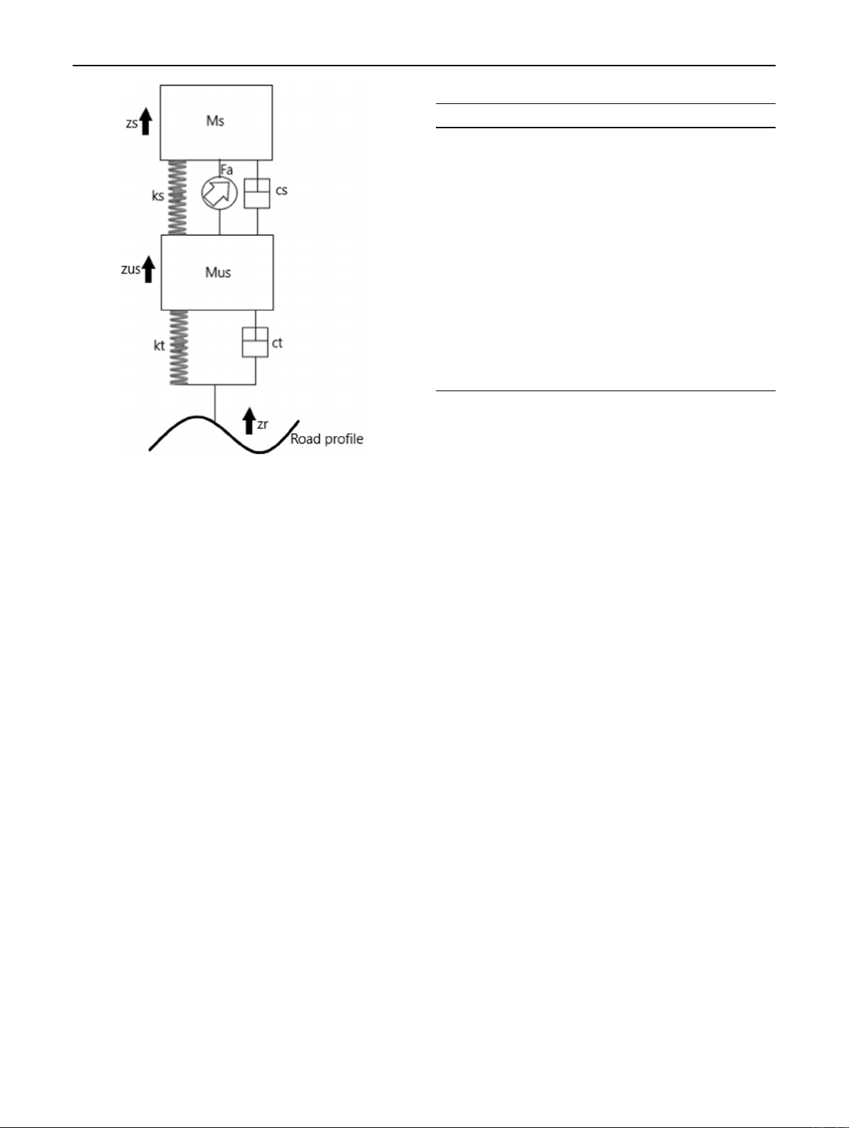
Active Suspension System
Data and Assumptions
The 2-DOF quarter vehicle model with an active suspen-
sion system is shown in Fig. 1. The definitions of the
coefficients and their values are given in Table 1. The
model is subjected to road bumps, which are modeled in
further sections. Plus, all the stiffness coefficients and
damping constants are linear. According to Iftikhar [17],
the linear suspension system has lower sprung mass and
unsprung mass maximum displacement and setting time
when the step input is used as a road profile. Iftikhar
concluded that the sprung mass and unsprung mass maxi-
mum displacement show lower magnitudes in the nonlinear
system than the linear one when the vehicle hits a non-
continuous sinusoidal road profile. However, according to
the Iftikhar’s results, in the noncontinuous sinusoidal
bump, the setting times for both masses in the linear system
are less than nonlinear ones. Assuming that the road is
perfectly flat after five seconds and to gain a low setting
time after the vehicle goes over bumps, the author opted for
a linear system based on the details mentioned earlier.
Table 1shows the quarter car model’s data and its
actuator in the suspension system [18,19]. Another
assumption which is made in this problem is as below:
Maximum suspension travel: 10cm
Vehicle’s constant speed: 12:5m=s
The maximum output voltage of the PID controller:
20volt
Maximum spool valve displacement: 2cm
Servo valve time constant: 4:50 103second
The top speed of the hydraulic cylinder: 0:6255m=s
Voltage to ampere conversion gain:
KVA ¼1:00 103A=V
Meter to voltage conversion gain: KMV ¼100V=M
Equations governing the problem
The problem to be studied is shown in Fig. 1. The goal is to
apply the desired value of force or pressure trajectory to the
system when the vehicle is subjected to a road bump. The
desired force will be applied to both the car’s wheel and
body, and this action will cause movement of the vehicle
body to the desired amount. This force is produced via a
double-acting hydraulic cylinder driven by a four-way
spool valve shown in Fig. 2. The servo valve has its closed-
loop control system, and it acts as a subsystem in the
overall control system. In Fig. 2, the position of the piston
is measured by a position transducer, which further gives a
voltage signal (uf) as an input to the servo amplifier. Then,
Fig. 1 Quarter car active suspension system
Table 1 Data for quarter car model with an active suspension system
Coefficient Definition Value Unit
mus Unsprung mass 41.5 kg
msSprung mass 241.5 kg
ksSpring stiffness 6:0103N=m
ktTire stiffness 1:4104N=m
csSpring damping 300 N:s=m
ctTire damping 1500 N:s=m
zus Unsprung mass displacement m
zsSprung mass displacement m
zrRoad profile m
ApActuator piston area 1:1103m2
VtThe total volume of the chamber 1:1104m3
Ctp Total leakage coefficient 1:01011 m5=N
beEffective bulk modulus 8:0108N=m2
PsSupply pressure 2:10 107N=m2
123
J. Inst. Eng. India Ser. C (August 2022) 103(4):1001–1011 1003
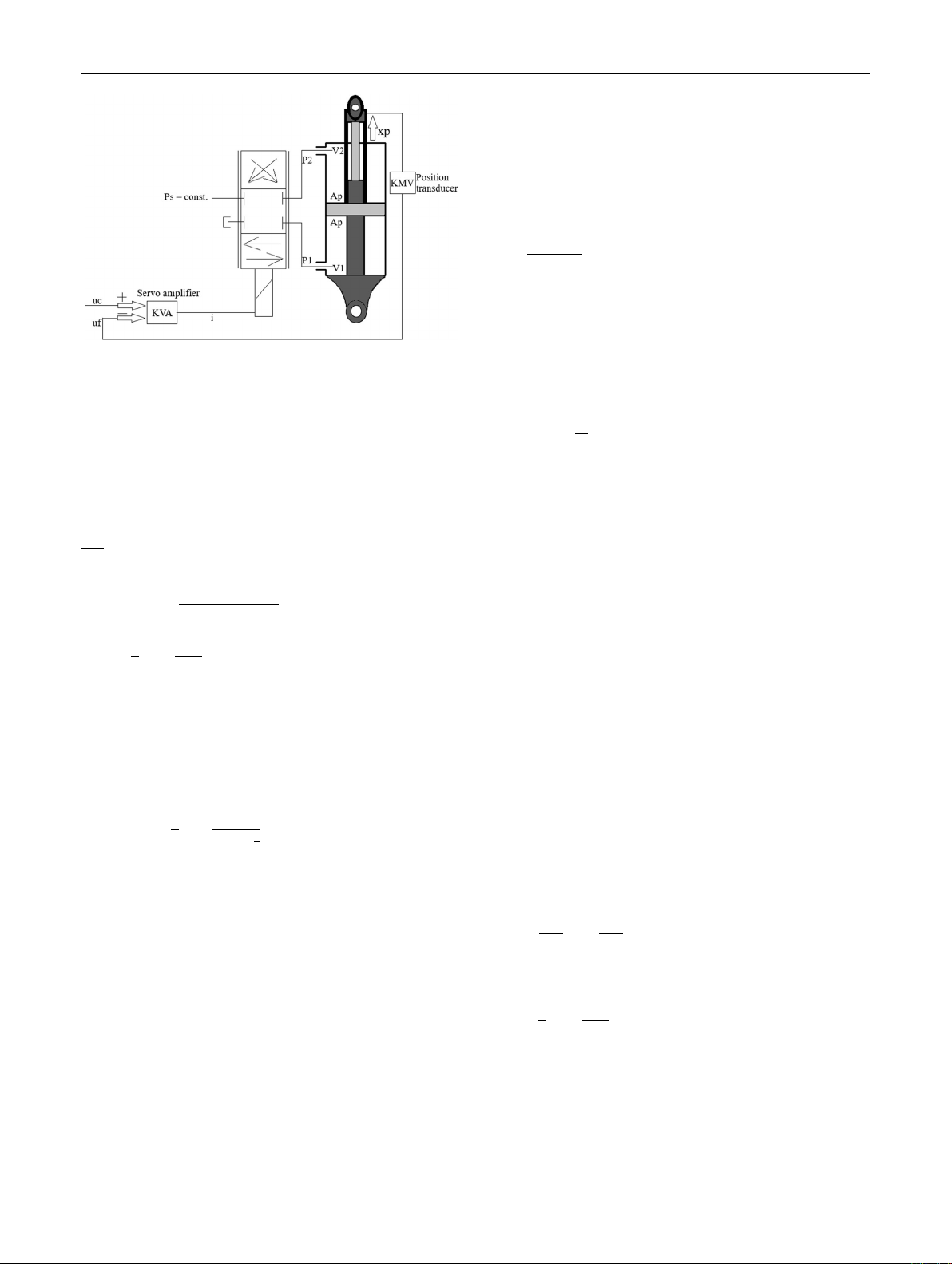
the servo amplifier will compare the command signal (uc)
with the feedback signal (uf), and the resultant error is
gained with the factor (KVA). However, with having a PID
controller in the system, the resulting error signal gains
with PID parameters.
The differential equations governing the actuator
dynamics are given as follows [20]:
Vt
4be
_
PL¼Ap
_
xpCtpPLþQL;ð1Þ
QL¼Cdwxvffiffiffiffiffiffiffiffiffiffiffiffiffiffiffiffiffiffiffiffiffiffiffiffiffiffiffiffiffiffi
Pssgn xv
ðÞPL
q
s;ð2Þ
_
xv¼1
sxvþKVA
su;ð3Þ
where xpis the actuator piston displacement, QLis the
load flow, Cdis the discharge coefficient, wis the spool
valve area gradient, xvis the spool valve position, qis the
fluid density, sis the servo valve time constant, KVA is the
voltage to ampere conversion gain, and uis the voltage
signal. The PID controller has the transfer function as:
UsðÞ¼PþI1
sþDN
1þN1
s
;ð4Þ
where Pis the proportional gain, Iis integral gain, D is
derivative gain, and Nis filter coefficient.
According to Ref. [13], the nominal load flow gives a
valve efficiency of gsv ¼0:67, where gsv is equal to PL=Ps.
Hence, in this problem, the maximum load pressure is
PLmax ¼1:407 107N=m2. However, in practice, the valve
efficiency will be lower when the valve leakage flow is
considered. Referring to the approach to force control for
electro-hydraulic systems studied by Alleyne [21], the
expression ffiffiffiffiffiffiffiffiffiffiffiffiffiffiffiffiffiffiffiffiffiffiffiffiffiffiffiffiffiffi
Pssgn xv
ðÞPL
pis seldom to zero when the
system operates smoothly since load pressure is seldom
close to zero. Alleyne’s claim is in contrast to the Rydberg
[9] state, which proves that the maximum load pressure is
2=3Psfrom the efficiency / load pressure derivative equal
to zero. Hence, by opting to PLmax ¼2=3Ps, the DPv¼
PsPL
ðÞ¼6:93 106N=m2the servo valve nominal flow
for mentioned pressure difference is defined as below:
QL¼QN¼Kqxv¼Apvmax;ð5Þ
where the valve flow gain can be written as Eq. (6)
which is written as:
Kq¼Apvmax
xv
;ð6Þ
where Eq. (2) is not used to obtain flow gain since the top
speed of the piston was given. Plus, the maximum actuator
speed value is an assumption given in this paper since the
values for the discharge coefficient, the spool valve area
gradient, and the exact maximum magnitude of load
pressure are not clear. Finally, by referring to the data,
assumptions, and Eq. (6), the valve flow gain becomes
Kq¼0:0344 m2
s.
The active suspension system applies a certain amount
of force to the wheel (unsprung mass) and body (sprung
mass), which the overall control system needs to reach the
desired input. The equations of motion based on Newton’s
law are given as:
Ms
€zsþkszszus
ðÞþcs
_zs_zus
ðÞFa¼0;ð7Þ
Mus
€zus þct
_zus _zr
ðÞþkszus zs
ðÞþcs
_zus _zs
ðÞ
þktzus zr
ðÞþFa
¼0;ð8Þ
where zris road profile, and Fais actuator force
(Fa¼ApPL).
Further, by assuming zs¼x1,zus ¼x3,zr¼xr,PL¼x5
and xv¼x6, Eq. (1), Eq. (3), Eq. (7), and Eq. (8) can be
rewritten in the form of first-order differential equations as
below:
_
x1¼x2;
_
x2¼ks
Ms
x1cs
Ms
x2þks
Ms
x3þcs
Ms
x4þAp
Ms
x5;
_
x3¼x4;ð9Þ
_
x4¼ctþcs
Mus
x4þct
Mus
_
xrþks
Mus
x1þcs
Mus
x2ksþkt
Mus
x3
Ap
Mus
x5þkt
Mus
xr;
_
x5¼ax2x4
ðÞbx5þcffiffiffiffiffiffiffiffiffiffiffiffiffiffiffiffiffiffiffiffiffiffiffiffiffiffiffiffiffi
Pssgn x6
ðÞx5
p
x6;
_
x6¼1
sx6þKVA
su;
where a¼4Abe=Vt;b¼4Ctpbe=Vt;and c¼
4Cdbew=Vtffiffiffi
q
p
:
Equation (9) is the simplified representation of actuator
dynamics and is modeled in the next section. Before
Fig. 2 Symbol circuit of a position servo
123
1004 J. Inst. Eng. India Ser. C (August 2022) 103(4):1001–1011
modeling the system, it is also necessary to define road
profile xraccording to Eq. (9). This paper describes road
profiles as the street bumps assumed to be continuous
sinusoidal and random irregular shape bumps. Therefore,
besides this study’s ideal sinusoidal street profile, a random
irregular road profile is also used, representing a more
realistic street bump.
Active Suspension Control System Design
In this section, the design of the active suspension control
system is studied. Many methods exist to design an active
suspension system, such as nonlinear modeling a vehicle
suspension using the LPV technique reviewed by Gaspar [22].
The goal of using the LPV method by Gaspar was to compose
a nonlinear suspension controller that can highlight a distinct
performance objective, depending on the size of the suspen-
sion deflection. While the suspension deflection is small, the
controller should concentrate on passenger comfort. When the
displacement limit is approached, the controller should stop
the suspension deflection from passing this limit. The LPV
method is an excellent approach to control nonlinear systems
using a family of linear controllers. However, a significant
shortcoming of the classical gain scheduling method is that
satisfactory performance, and in some matters, yet stability is
not insured at operating states other than the design points
[23]. Considering that the system presented in this paper is
linear, it is more promising to use a numerical simulation
method using SIMULINK in MATLAB to design and control
the active suspension system.
The SIMULINK environment provides a large range of
designing and controlling tools and apps, which are helpful
to satisfy the system’s stability and performance. Regard-
ing controlling an active suspension system, recent works
such as Mudduluru [12] conclude that active suspension
controlled by the PID controller provides a better response
than a passive system. The application of the PID con-
troller for a quarter and full car model, which is studied by
the researchers [12], shows a significant reduction in mass
sprung displacement.
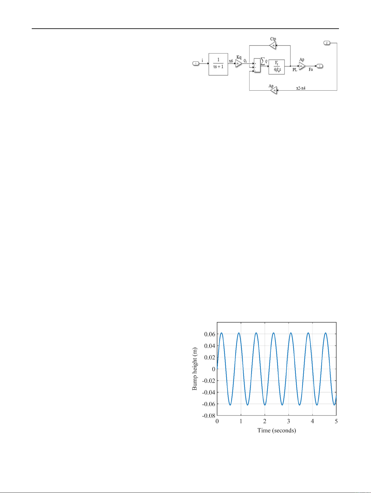
Actuator Modeling
The actuator in the active suspension system is considered
double-acting by a four-way spool valve. Figure 3shows
the subsystem of the hydraulic cylinder with its valve
inside the overall control system. The dynamic models of
the valve and hydraulic cylinder are obtained via consid-
ering Eq. 8and data and assumption. The force that is
obtained by the actuator is applied on both sprung mass and
unsprung mass, which can affect the vehicle’s body
displacement.
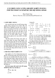
Road Profile Modeling
Figures 4and 5indicate the road profiles xrdesigned for
this study using SIMULINK. The shape of the bump is
sinusoidal with a 0.062 m amplitude. The assumed bumps
maximum heights prevent the suspension deflection from
approaching its limit, which is 10 cm.
General Modeling of the Control System
Considering the overall dynamic equations of the active
suspension system given in Eq. (8) and the road profiles xr,
shown in Figs. 4and 5, the final model of the system is
shown in Fig. 6. In this control system, the road profile
signal acts as a disturbance signal. The actuator itself is a
subsystem inside the overall system, and it aims to generate
the necessary force to apply to the vehicle body and the
wheel. The actuator force is obtained via a PID controller,
which commands the valve by a current signal. Further, the
displacement of the spool valve caused by the current
signal gives a certain amount of oil rate inside the cylinder.
Then, the hydraulic cylinder converts fluid energy to
kinetic energy with the movement of the piston. Finally, a
shaft connected to the piston moves upward and down-
ward, leading to the vehicle’s body movement.
Fig. 3 Block diagram for a valve-controlled cylinder
Fig. 4 Continuous sinusoidal road profile xr
123
J. Inst. Eng. India Ser. C (August 2022) 103(4):1001–1011 1005


![Giáo trình Thực hành Truyền động điện Trường Đại học Bà Rịa - Vũng Tàu [Mới nhất]](https://cdn.tailieu.vn/images/document/thumbnail/2026/20260310/hoaphuong0906/135x160/11121773283865.jpg)
![Giáo trình Thực hành SCADA Trường Đại học Bà Rịa - Vũng Tàu [Mới nhất]](https://cdn.tailieu.vn/images/document/thumbnail/2026/20260310/hoaphuong0906/135x160/94061773283866.jpg)
![Tài liệu học tập La bàn từ [mô tả/định tính]](https://cdn.tailieu.vn/images/document/thumbnail/2026/20260310/hoaphuong0906/135x160/25191773287376.jpg)

![Tài liệu học tập Thiết kế hệ thống nhúng [mới nhất, đầy đủ]](https://cdn.tailieu.vn/images/document/thumbnail/2026/20260305/hoatulip2026/135x160/37051773135929.jpg)


![Giáo trình Điều khiển khí nén thuỷ lực Phần 2: [Mô tả/Chủ đề cụ thể của phần 2]](https://cdn.tailieu.vn/images/document/thumbnail/2026/20260302/camtucau2026/135x160/11911772768225.jpg)
![Giáo trình Điều khiển khí nén thuỷ lực Phần 1: [Mô tả/Định tính thêm nếu cần]](https://cdn.tailieu.vn/images/document/thumbnail/2026/20260302/camtucau2026/135x160/51511772768225.jpg)
![Giáo trình Điều khiển số Phần 2: [Thêm từ khóa mô tả nội dung chương trình]](https://cdn.tailieu.vn/images/document/thumbnail/2026/20260302/camtucau2026/135x160/37201772766913.jpg)
