Automatic.a,
Vol. 10, pp. 405-412. Pergamon Press, 1974. Printed in Great Britain.
The Effect of Feedback on Linear Multivariable Systems*
L'Effet de R&roaetion sur les Syst~mes Lin6aires multivariables
Der EinfluB der Rtickf'tihrung auf lineare multivariable Systeme
B~HaHHe o6paTnofi CBg3H sa ~HHeflmae MHOronapaMerpHqeCxl~e CHffl~M
D. Q. MAYNEt
Certain basic operations, the most important being the determination of the effect oJ
feedback on a matrix transfer function, can be performed
algebraically
rather than
numerically at specific frequencies, enhancing the power of existing procedures for
designing linear multivariable control systems.
Statutory--This paper describes effective
algebraic
procedures
for performing certain operations on matrix transfer
functions, the most important being the calculation of the
effect of feedback. Such operations are required, for
example, in designing, sequentially, controllers for linear
multivariable systems. Previous papers have described
algorithms for performing these operations numerically at
specific frequencies to obtain, for example, the closed-loop
matrix frequency response, in numerical form. However, if
algebraic solutions, which are matrix transfer functions
whose elements are rational functions, are required, naive
use of standard formulae must be avoided, since they result
in rational functions of needlessly high degree. This paper
shows how this needless increase in the degree of the
rational functions may be avoided, thus yielding effective
algebraic procedures for the operations considered. Although
the results are of interest in their own right, a brief resume
of a specific procedure, the sequential return difference
method, for designing linear multivariable control systems
which utilises these results, is given.
1. INTRODUCTION
IN DVSIG~N(3 linear multivariable systems [l]
several basic operations recur: firstly, calculating
the effect of feedback on a matrix transfer function;
secondly, calculating the product of two matrix
functions when designing pre- and post-
compensators; thirdly, given the closed-loop
transfer function relating the output to one input,
determine the transfer function relating the
output to another input. These operations are
easily performed numerically at specific frequencies
[l], essentially a frequency response determination.
However if
algebraic
solutions, which consist of
matrix transfer functions whose elements are
sational functions, are required, then naive use of
* Received 23 July 1973; revised 15 January 1974. The
original version of this paper was not presented at any
IFAC meeting. It was recommended for pubfication in
revised form by Associate Editor H. Kwakernaak.
1' Present address: Department of Computing and Control,
Imperial College of Science and Technology, Exhibition
Road, London, SW7
2BT.
standard formulae results in polynomials of very
high degree. This paper shows how needless
increase in the degree of these polynomials can be
avoided, thus yielding an effective
algebraic
pro-
cedure for the above three operations. To show the
relevance of these operations a brief resume of a
design procedure, the sequential return difference
method, which utilises these operations is given in
§2. The algebraic procedures, which are of interest
in their own right, are then presented in §3, ~4
and §5.
2. THE DESIGN OF LINEAR MULTIVARIABLE
SYSTEMS
Let the r × r transfer function matrix of the plant
to be controlled by
Gp(s).
It is desired to choose a
(feedback) transfer function matrix
GI(s )
so that
the system:
y(s)=O,(s)u(s) (I)
u(s)=C/(s)D, ~(s)- y(s)]
(2)
where y is the output and Yd the system reference
input which represents the "desired" output,
satisfies certain design criteria. Equations (1) and
(2) yield:
y(s)=R(s)y.(s)
(3)
where
and
R(s)=[T(s)]- ~ O~(s)~ f(s)
(4)
T(s) is the matrix return difference and
R(s)
the
closed loop transfer function Yd to y. The basic
design criteria are:
405
406 D.Q. MAY~
(i) Stability
(ii) Attenuation of disturbances, insensitivity to
parameter variation, i.e. system perfor-
mance.
Other criteria having importance in some appli-
cations are:
(iii) Low interaction
(iv) Maintenance of stability if certain specified
parameters change, within a prespecified
range, because of, for example, com-
ponent failure, i.e. system security.
The important factors relevant to these criteria
are as follows:
(i)
Stability
Let the open-loop system, plant and controller,
be described by:
y(s)----G gs)u(s) + d(s)
(r)
then the response of the closed-loop system is:
y(s) :R(s)yd(s ) +
[T(s)]-
'd(s)
(3')
so that the effect of the disturbance in the frequency
band [0, co¢] is small if
HT-'(i(o)[] _<1 for all
(o~[0,
(oc].
(13)
This requires feedback from all r outputs such that
the loop gain
Gp(ico)G¢(ico)
is large compared with
1, for all o~[0, COc], in the sense that
[T(ico)]- 1 = [I, +
Gp(ico)G:(i¢o)]-I
-
G 7'(ko)Gp
l(ito)
(14)
i.e. such that the feedback is "tight".
= A x + Be. (6)
y=Cx.
(7)
The transfer function e to y is:
Gp(s) Gf(s) = C(s/- .4 ) -
' O
( 8 )
and the open-loop characterist;c polynomial is:
po(S)=lsI-A I.
(9)
The closed-loop system satisfies (6), (7) and:
e=y d-y
(10)
so that:
:c:(A -BC)x + Byd.
(11)
The closed-loop characteristic polynomial is:
m(s)=lsI-A + BC I.
(12)
The following result is well known [1]:
Proposition 1.
IT(s)[
=p#)lpo(s).
Hence the closed-loop system is stable if the
roots of
Ir(s)l
lie in the open left-half plane. This
cart often be achieved by single-loop feedback;
multivariable feedback may not be necessary for
stability.
(2)
Attenuation of disturbance
If a disturbance d is present so that (1) becomes:
(3)
Low interaction
if the feedback is "tight" in the band [o,c0d, then:
R(ico) = [T(ito)]-lGp(ico)Gf(ico) - I
for all coe[o,c%], so that "tight" feedback auto-
matically results in low interaction at low fre-
quencies.
As
s~ov Gp(S)Gs(s)oO
if, as is usual,
G(s)Gi(s )
has the representation (6), so that, as s-* ov :
n(s)~6,(s)CAs)
and low interaction at high frequencies, if required,
can be obtained by choosing
GI(s )
so that
Gp(s)GI(s)-~
a diagonal transfer function matrix.
(4)
Security
Let
T~(s)
denote the matrix return difference
corresponding to a parameter vector, of dimension
q, having value ct, and suppose stability is required
for all r, eA = RL Then the system remains stable
for all ~teA if the roots of IT'(s)[ lie in the open
left half plane for all ~teA.
In achieving these objectives the following result
due to ROS~Nm~OCK [5] is crucial.
Proposition 2. Let G:(s)
be a non s;ngular rational
transfer function matrix. Let all the poles of
G/(s)
and all the zeros of
I As)l
lie in the open left half
plane. Then,
G/(s)
can be expressed as the product
PG ,(s)K(s)
where
(a) P is a (column) permutation matrix
(Iel=+l).
(b)
Gc(s )
is the product of elementary column
operations which are of the form add
The effect of feedback on linear multivariable systems 407
• (s)x column i to column j, ~ being a
rational polynomial function having all ;ts
poles in the open left half plane, so that
(C)
K(s)
is a non-singular diagonal matrix,
whose diagonal elements have all their poles
and zeros in the open left half plane.
Hence the control structure of Fig. 1, where the
compensator
G,(s)
satisfies
IG,(s)l-
1 and the con-
troller
K(s)
is diagonal is sufficiently general
provided that prior column interchanges in
Gp(s)
are permitted.
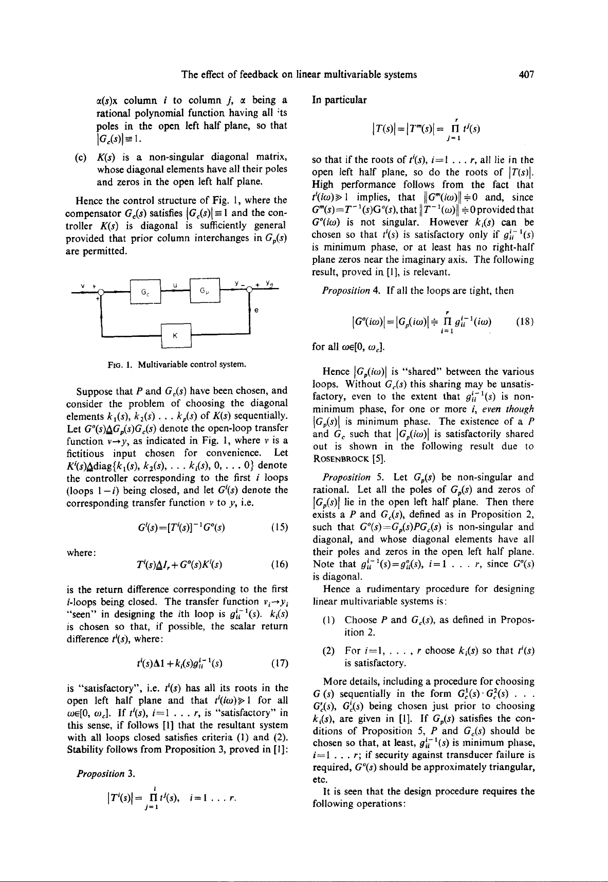
Flo. I. Multivariable control system.
+ Yg
e
Suppose that P and
G~(s)
have been chosen, and
consider the problem of choosing the diagonal
elements kl(S),
kz(s).., kp(s)
of
K(s)
sequentially.
Let
G°(s)AGp(s)Gc(s)
denote the open-loop transfer
functiort
v~y,
as indicated in Fig. 1, where v is a
fictitious input chosen for convenience. Let
KJ(s)Adiag{kt(s),
k2(s),..,
k~(s), 0 ....
0} denote
the controller corresponding to the first i loops
(loops 1- i) being closed, and let
Gi(s)
denote the
corresponding transfer function v to y, i.e.
at(s)
= [Ti(s)] -
aG°(s)
(15)
where:
Ti(s)A_I, + G°(s)K~(s)
(16)
is the return difference corresponding to the first
/-loops being closed. The transfer function
v~--,y~
"seen" in designing the ith loop is gl/-l(s),
k~(s)
is chosen so that, if possible, the scalar return
difference
tt(s),
where:
t'(s) A 1 + k,(s)g171
(s) ( l 7)
is "satisfactory", i.e.
t~(s)
has all its roots in the
open left half plane and that d(ito)~>l for all
toe[0, o~c]. If
d(s),
i----I . . . r, is "satisfactory" in
this sense, if follows [1] that the resultant system
with all loops closed satisfies criteria (1) and (2).
Stability follows from Proposition 3, proved in [1]:
Proposition 3.
l
Ir'(s)l= n
j=l i=l .. ,r.
In particular
Iz(s)l=lT'(s)[= fi
j=l
so that if the roots of ti(s), i=l ... r, all lie in the
open left half plane, so do the roots of IT(s)l.
High performance follows from the fact that
tl(iog)~>
1 implies, that
IIo'(/,o)lr :--0 and,
since
G'(s) =T-
l(s)G
°(s),
that
II T- 1 o )11
- 0 provided that
G°(io)
is not singular. However
ki(s)
can be
chosen so that
t~(s)
is satisfactory only if g17 l(s)
is minimum phase, or at least has no right-half
plane zeros near the imaginary axis. The following
result, proved irt [1], is relevant.
Proposition
4. If all the loops are tight, then
[G°(ioO[=[Go(ioOI - n aiT'(io) (18)
i=1
for all o~e[0, Wc].
Hence
IGp(kO)l
is "shared" between the various
loops. Without
Go(s)
this sharing may be unsatis-
factory, even to the extent that gi71(s) is non-
minimum phase, for one or more
i, even though
IGv(s)[
is minimum phase. The existence of a P
and G c such that
IO~(i~o) I
is satisfactorily shared
out is shown in the following result due to
ROSENBROCK [5].
Proposition
5. Let
Gp(s)
be non-singular and
rational. Let all the poles of
Gv(s )
and zeros of
Ic.(s)l
lie in the open left half plane. Then there
exists a P and
Go(s),
defined as in Proposition 2,
such that
G°(s)--Gp(s)PGc(s)
is non-singular and
diagonal, and whose diagonal elements have all
their poles and zeros in the open left half plane.
Note that i-1 o
g, (s)=9,(s),
i=1 . .. r, since
G°(s)
is diagonal.
Hence a rudimentary procedure for designing
linear multivariable systems is:
(1) Choose P and
Go(s),
as defined in Propos-
ition 2.
(2) For i=1 ..... r choose
ki(s)
so that
ti(s)
is satisfactory.
More details, including a procedure for choosing
G (s) sequentially in the form
G~(s)'G2(s) . . .
G~(s), Gic(s)
being chosen just prior to choosing
k~(s),
are given in [1]. If
Gp(s)
satisfies the con-
ditions of Proposition 5, P and
G~(s)
should be
chosen so that, at least, gli t(s) is minimum phase,
i=1 . . . r; if security against transducer failure is
required,
G°(s)
should be approximately triangular,
etc.
It is seen that the design procedure requires the
following operations:
408 D.Q. MAYNE
(1)
Given
G~-'(s)
and k'(s) determine
Gl(s)
where:
~'(s)=[I~(s)]- 'G'- '(s)
(19)
G°(s) = C[sI- A + knb .p% .]- 'B
(26)
where %. is the pth row of C, and b .o the pth
column of B. Hence:
7~(s)
=
1 + kl(s)ff![" X(s)er
(20)
G'(s)=[~e(s)] -
'G o- '(s)
(27)
where
g!~l(s)
is the ith column of Gi-l(s)
and et is the ith column of I,.
(2) Given G'- J(s) and
G~(s)
calculate G'-
X(s)G~(s).
(3) Given
Gin(s),
the dosed loop transfer
function
v-}y,
calculate
which, in this ease, reduces to:
G°(s) = G p- '(s) -- kog ~- l(s)gP.- l(s)/to(s)
(28)
where go. denotes the pth row of G, and:
to(s)A 1 + knO ~- 1(s) (29)
R(s)=G"(s)K(s)
the dosed-loop transfer function
y,~y.
is the scalar "return difference" for the pth loop.
The "open-" and dosed-loop characteristic poly-
nomials are, respectively:
The following sections show how these operations
can be performed algebraically. Previously [1,5]
design procedures were implemented by per-
forming these operations numerically at specific
frequencies. Algebraic use of the formulae
developed for numerical evaluation results in
rational functions of needlessly high degree.
3. THE EFFECT OF FEEDBACK ON MATIRX
TRANSFER FUNCTIONS
Let S o- 1, the system prior to the dosing of the
pth loop, be described by:
Yc(t) =Ax(t) + Bu(t)
(21)
y(t)=Cx(t)
(22)
where {A, B, C} is not necessarily minimal.
x(t)eR"
is the state at time
t, u(t)¢R m
the input and
y(t)eR"
the output. The r × m transfer function u
to y is:
Go- ~ (s) = C(sl - A) - ~ B.
(23)
Assume now that the pth loop is closed i.e.
u(t) = v(t)- Ky(t)
(24)
where
K=kpD,
and
DeR m~"
is defined by:
do=O
if
i~p orjv~p
doo= l.
For this structure, the matrix return difference
is:
T°(s) = I, + G °-
t(s)K
= l, + k~:- '(s)g,
(25)
where
g .e
denotes the pth column of G and e o the
pth column of
I,.
It is well known that the do,d-
loop transfer function v to y is:
pf-'(s)~J81-,41 (3O)
,f(8)~lst- X+ k,b.,c,. I . (31)
It is well known [1] that
t,(s) = p~(s)/p~- l(s)
(32)
The lowest common denominator of the elements
GP-I(s)
clearly divides pP~(s), so that GP-~(s)
may be expressed as:
G p- l(s) = N °- l(s)/pP- 1(8).
(33)
Similarly,
GP(s)
may be expressed as:
Gn(s)
=
N°(s)/p~(s)
(34)
where
N °-
1(8) and
No(s)
are polynomial matrices.
pff-~ and p~ have the same degree n: However
naive application of (28) yields a matrix whose
elements have numerator and denominator poly-
nomials of degree between n and 2n. This difficulty
is overcome by:
Proposition
6. IfK=knDthen
GO(s)-- NO(s)/p~(s)
is given by:
(i)
p,,(s) = pf- '(s) + kon;f ~(s)
(35)
(ii) Ififfiporjffip
nt/s) f nf;"(s).
(36)
Otherwise:
rills) ffi nf: '(s) + k,8~- ~(s) (37)
where
The effect of feedback on linear multivariable systems
F
nwWw'(s) n~"
1(s) 1 I
¢-'(s) Lnf,-'(s) nr,;1(s).l ~-'~';)
(3s)
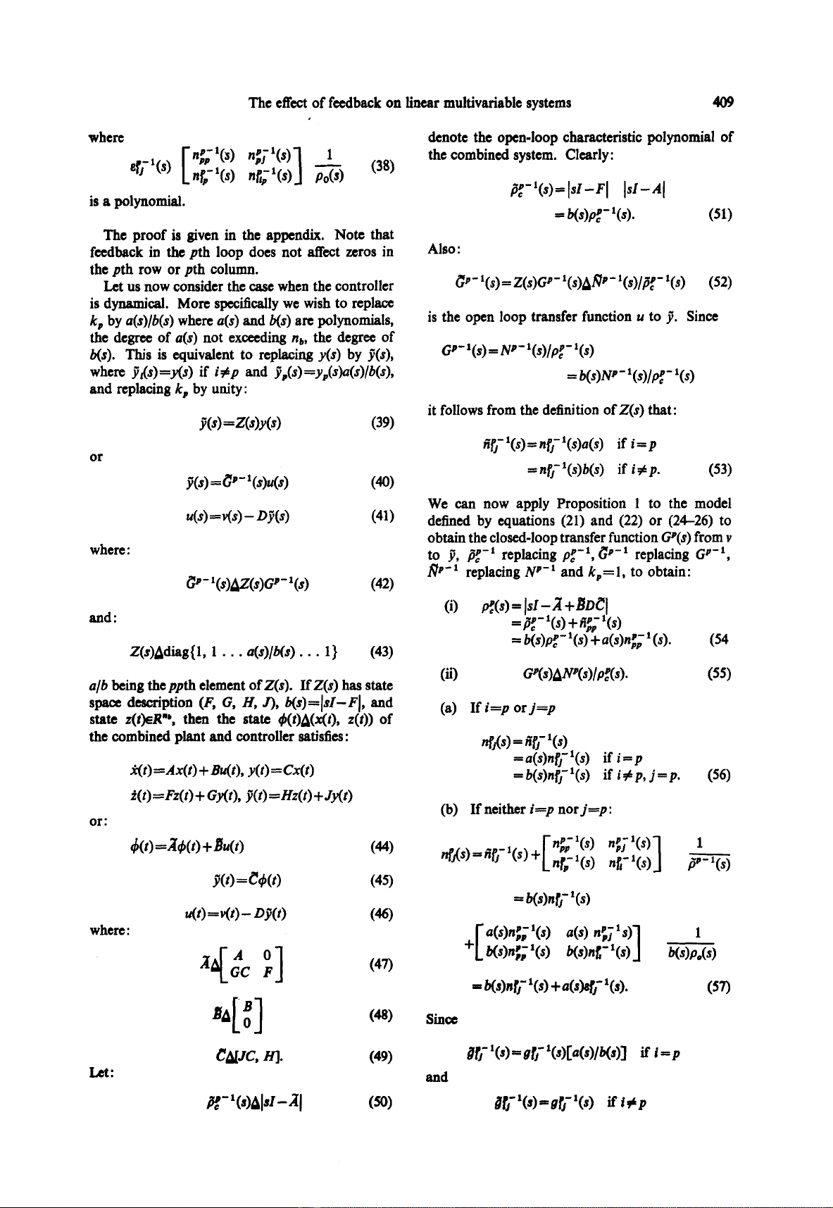
is a polynomial.
The proof is given in the appendix. Note that
feedback in the pth loop does not affect zeros in
the pth row or pth column.
Let us now consider the case when the controller
is dynamical. More specifically we wish to replace
k, by
a(s)/b(s)
where
a(s)
and b(s) are polynomials,
the degree of
a(s)
not exceeding ne, the degree of
b(s). This is equivalent to replacing
y(s)
by ~(s),
where ~t(s)fy(s) if
i~p and ~,(s):yr(s)a(s)/b(s),
and replacing k w by unity:
or
.~(s)=Z(s)y(s)
(39)
)(s)=Gp- ' (s)u(s) (4o)
whe~:
u(s) =~(s)- D p(s) (41)
(42)
and:
#,-1(s):z(s)~,-1(s)
Z(s)Adiag{l, 1 ...
a(s)/b(s)...
I} (43)
Mb being the ppth
element of
Z(s).
If Z(s) has state
space description
(F, G, H, Y), b(s)----[sl-F], and
state z(t)eR",
then the state
O(t)A(x(t),
z(t)) of
the combined plant and controller satisfies:
~t)=Ax(t) +
S~(t), y(t)=Cx(O
~(o=ez(t) + ~.r(t), )(t)=Hz(t) + Jy(t)
d(t) =2~(t) +
gu(t) (44)
y(t)=~(t) (45)
or:
whe~:
,~t)=v(t)- Dp(t)
(46)
~AI'./C, H].
(49)
4O9
denote the open-loop characteristic polynomial of
the combined system. Clearly:
Ist-AI
= b(s)~-'(s). (51)
Also:
~'- ~(s) ffi Z(s)G,- ~(s)~q'- '(s)/~f- ~(s) (52)
is the open loop transfer function u to ~. Since
G'- '(s) = IV" - l(s)/p~- l(s)
= b(s)N,- '(s)/~- '(s)
it follows from the definition of Z(s) that:
6~-l(s)--'n~-l(s)a(s)
if
i=p
=n~-~(s)b(s)
if
i~p.
(53)
We can now apply Proposition 1 to the model
defined by equations (21) and (22) or (24--26) to
obtain the closed-loop transfer function
UP(s)
from v
to ~, #P- 1 replacing PeP- 1, ~p- 1 replacing G p- 1,
~tp- 1 replacing N p- 1 and k, = 1, to obtain:
(i) ~(s) ffi
Isl- t~
+BD~[
ffi #~'- ,(s ) + ,~'; '(s)
= b(s)p~c- l(s) + a(s)n~; 1 (s).
(54
(ii)
G#(s)ANW(s)/ p~(s). (55)
(a)
If i=p or j=p
,,G(s) ffi,~lT'(s)
~a(s)n~-l(s)
if
i=p
~b(s)nf71(s)
if
iCp, jfp.
(56)
(b) If neither
i=p
norj=p:
, xs,
1
, ,, "TLnr,-'(s)
n[-'(s)J
#'-'(s)
=b(s)n~-'(s)
,.roe,),,;.',,) o(,)
n;;'s)l '
Lb(s)n';'(s) b(s)nF'(s)] b(s)p.(s)
= b(s)n~- l(s) + a(s~- ~(s).
(57)
Let:
Since
and
~-'(s)~kl-;q (5o) Off '(s)=gff '(s) if ~,~ p


![Bài giảng Vi điều khiển Nguyễn Huy Hoàng: Tổng hợp kiến thức [Chuẩn nhất]](https://cdn.tailieu.vn/images/document/thumbnail/2026/20260316/hoatrami2026/135x160/72211773806757.jpg)


![Bài giảng Tự động hoá thiết bị điện [chuẩn nhất]](https://cdn.tailieu.vn/images/document/thumbnail/2026/20260312/hoabattu2026/135x160/61691773631881.jpg)
