
ISA Transactions 51 (2012) 550–558
Contents lists available at SciVerse ScienceDirect
ISA Transactions
journal homepage: www.elsevier.com/locate/isatrans
Decentralized PI/PID controllers based on gain and phase margin specifications
for TITO processes
D.K. Maghadea, B.M. Patreb,∗
aDepartment of Instrumentation and Control Engineering, Vishwakarma Institute of Technology, Pune-411037, India
bDepartment of Instrumentation Engineering, Shri Guru Gobind Singhji Institute of Engineering and Technology, Vishnupuri, Nanded-431602, India
article info
Article history:
Received 5 January 2011
Received in revised form
2 January 2012
Accepted 21 February 2012
Available online 23 March 2012
Keywords:
Decentralized controller
Decoupled system
Empirical modeling
Interactive processes
Model order reduction
Real time application
abstract
In this paper, a decentralized PI/PID controller design method based on gain and phase margin
specifications for two-input–two-output (TITO) interactive processes is proposed. The decouplers are
designed for systems to minimize the interaction between the loops, and the first order plus dead time
(FOPDT) model is achieved for each decoupled subsystem based on the frequency response fitting. An
independent PI/PID controller is designed for each reduced order decoupled subsystem to obtain the
desired gain and phase margins, and the performance is verified on the original interactive system to
show the effectiveness of the proposed design method for the general class of TITO systems. Simulation
examples are incorporated to validate the usefulness of the presented algorithm. An experimentation is
performed on the Level–Temperature reactor process to show the practical applicability of the proposed
method for the interactive system.
©2012 ISA. Published by Elsevier Ltd. All rights reserved.
1. Introduction
Many of the industrial processes have multi-input–multi-
output (MIMO) dynamics with interaction among the input–output
variables. In most of the industrial processes, decentralized con-
trol is used instead of multivariable centralized control since the
decentralized controller is simple to design, easy to tune, imple-
ment and maintain [1]. In the literature, the multi-loop PI/PID
control using multiple single-input–single-output (SISO) PI/PID
controllers is commonly used for controlling MIMO systems with
interaction [2]. The reason for using SISO PI/PID controllers for
multi-loop control is its simple structure, easy tuning and an abil-
ity to meet most of the control objectives [3–7]. However, due to
interactions, the design and tuning of centralized multi-loop con-
trollers is much more difficult compared with that of single-loop
controllers [8]. In centralized multi-loop controllers, since the con-
trollers interact with each other, the tuning of one loop cannot be
done independently. An extension of the controller design meth-
ods for a SISO system to multi-loop systems often affects the per-
formance and stability of the systems. Many methods have been
proposed, including the detuning method [9,10], sequential loop
closing method [11,12], relay auto-tuning method [13–17], and
∗Corresponding author. Tel.: +91 2462 269324; fax: +91 2462 229236.
E-mail addresses: bmpatre@yahoo.com,bmpatre@sggs.ac.in (B.M. Patre).
independent loop method [18,19] to take loop interactions into
account in the multi-loop controller design. In detuning big log
modulus method, first introduced by Luyben [9], each controller in
the system is designed based on the corresponding diagonal ele-
ment and ignore the interactions from other loops. The controllers
are then detuned considering interactions until some prescribed
limit is attained. The detuning methods are simple, but the loop
performance and stability of the system cannot be clearly defined
through the detuning procedures. In the sequential loop closing
method, the loops are closed usually from the fastest loop, one after
the other. The dynamic interaction of closed loop is taken into ac-
count while closing of next loop, and so on. However, the final con-
troller design may depend on the order by which the controllers
are designed, and iteration procedures are essential because clos-
ing the subsequent loops may alter the response of the previously
designed loops [18]. In the relay auto-tuning method, the relay
feedback technique is applied to the design of each correspond-
ing SISO controller [13]. The control loops are tuned sequentially
and the multi-loop control system is designed in a sequence of
SISO design problems. These methods considered the interaction
in a sequential, require minimum process information, but tuning
sequence has to be repeated for the correct sequence if the de-
sign sequence is not appropriate. In independent design methods,
SISO controllers are designed independently by using the defined
bounds to guarantee stability and performance. But, the detailed
information about the controller dynamics in other loops is not
used, the resulting performance may be poor [12].
0019-0578/$ – see front matter ©2012 ISA. Published by Elsevier Ltd. All rights reserved.
doi:10.1016/j.isatra.2012.02.006

D.K. Maghade, B.M. Patre / ISA Transactions 51 (2012) 550–558 551
The TITO systems are one of the most prevalent categories
of multivariable systems, because there are real processes of
this nature or because a complex process has been decomposed
into TITO process with nonnegligible interactions between its
inputs and outputs [20–23]. Decentralized PID controllers with
decoupler are most commonly preferred for TITO processes [21,22,
24–29]. The detail discussion on the decoupling approach for TITO
systems is given in [30]. Tavakoli et al. proposed a decentralized
PI/PID controller for TITO systems based on nondimensional
analysis [21], while an ideal decoupler for the controller design
based on exhaustive search is presented by Nordfeldt and
Hägglund under the constraints on robustness and sensitivity
to measurement noise [22]. Jevtović and Mataušek presented
decentralized controller design method with ideal decoupler [23].
In this paper, simple decoupler plus decentralized PID controller is
proposed for general class of TITO systems. The frequency response
fitting based model order reduction technique is employed to get
FOPDT model of the each higher order decoupled subsystems.
An independently PI/PID controllers are designed for specified
gain and phase margins. The designed controller together with
decoupler are used to get the desired performance of the TITO
processes. The paper is organized as follows. Decoupler design
method is discussed in Section 2. In Section 3, a decoupled
higher order subsystem model is reduced into equivalent FOPDT
model. A PI/PID controller tuning formulas for FOPDT models are
presented in Section 4. To show performance and effectiveness
of proposed method two simulation examples are included in
Section 5. In Section 6, the discussion on empirical modeling of the
Level–Temperature reactor and the performance of the proposed
PI controller is included. Conclusions are drawn in Section 7.
2. The decoupling method
Let the TITO process is as follows
G(s)=g11(s)e−τ11sg12(s)e−τ12s
g21(s)e−τ21sg22(s)e−τ22s.(1)
The given process G(s)is decoupled using decoupler matrix [21].
To design decoupler matrix following two cases considered.
Case 1: The off-diagonal elements of G(s)have no RHP poles and
diagonal elements of G(s)have no RHP zeros.
The decoupler matrix is
D(s)=v1(s)d12(s)v2(s)
d21(s)v1(s) v2(s)(2)
with v1(s), v2(s), d12(s)and d21(s)as given in Eq. (3).
v1(s)=1, τ21 ≥τ22,
e(τ21−τ22)s, τ21 < τ22,
v2(s)=1, τ12 ≥τ11,
e(τ12−τ11)s, τ12 < τ11,
d12(s)= − g12(s)
g11(s)e−(τ12−τ11)s,
d21(s)= − g21(s)
g22(s)e−(τ21−τ22)s.(3)
Case 2: The diagonal elements have no RHP poles and off-diagonal
elements have no RHP zeros of G(s).
The decoupler in the form
D(s)=d11(s)v3(s) v3(s)
v4(s)d22(s)v4(s),
where,
v3(s)=1, τ22 ≥τ21,
e(τ22−τ21)s, τ22 < τ21,
v4(s)=1, τ11 ≥τ12,
e(τ11−τ12)s, τ11 < τ12,
d11(s)= − g22(s)
g21(s)e−(τ22−τ21)s,
d22(s)= − g11(s)
g12(s)e−(τ11−τ12)s.(4)
As shown in Eq. (5),H(s)is a diagonal matrix.
H(s)=G(s)D(s)=diag {h11(s), h22(s)}.(5)
The decoupled elements hii(s)are to be controlled through
decentralized PI/PID controllers kii(s), where i=1,2.
3. Model reduction
The dynamics of the elements hii(s)of H(s)are quite
complicated. A FOPDT model often reasonably describes the
process gain, overall time constant and effective dead time of
higher order processes [31]. In this section a FOPDT model lii(s)of
each elements hii(s)of H(s)is obtained as below
lii(s)=Kiie−Liis
Tiis+1,i=1,2.(6)
Three unknown parameters (Kii,Lii and Tii) in Eq. (6), need to be
determined, in order to obtain FOPDT model of hii. In this paper,
FOPDT model is obtained based on frequency response fitting at
two points, ω=0 and ω=ωcii, where ωcii is phase crossover
frequency [32].
lii(0)=hii(0),
|lii(jωcii)|=|hii(jωcii)|,
{lii(jωcii)}={hii(jωcii)}.(7)
As a result, the parameters of the FOPDT model can be calculated
using
Kii =hii(0),
Tii =K2
ii −|hii (jωcii)|2
|hii (jωcii)|2ω2
cii
,
Lii =π+tan−1(−ωciiTii)
ωciiTii
.(8)
4. The controller design method
The gain and phase margins (GPMs) are typical loop specifi-
cations associated with the frequency response [33]. The GPMs
have always served as important measures of robustness [34]. It
is known from classical control that phase margin is related to the
damping of the system, and can therefore also serve as a perfor-
mance measure [33]. The controller design methods to satisfy GPM
criteria are not new, and thus widely used [35–37]. In this paper,
simple formulas are developed to design the PI/PID controller to
meet user-defined gain margin and phase margin specifications.

552 D.K. Maghade, B.M. Patre / ISA Transactions 51 (2012) 550–558
4.1. PI tuning formula
Using definitions of GPM, following set of equations can be
written
arg lii(jωpii)kii(jωpii)= −π, (9)
Amii =1
lii(jωpii)kii(jωpii)
,(10)
lii(jωgii)kii(jωgii)=1,(11)
φmii =arg lii(jωgii)kii(jωgii)+π, (12)
where Amii and φmii are GM and PM respectively. Also ωgii and ωpii
are gain and phase crossover frequencies. The kii(s)is PI controller
for FOPDT model lii as given in Eq. (13). The PI controller is
kii(s)=kPii 1+1
TIiis(13)
where, kPii and TIii are proportional gain and integral time
respectively.
From Eqs. (6) and (13), the open loop transfer function is
lii(s)kii(s)=kPiiKii (sTIii +1)
sTIii (sTii +1)e−Liis.(14)
For given process and GPM specifications, the PI controller
parameters and crossover frequencies can be obtained numerically
but not analytically because of the presence of the arctan function.
The arctan function is approximated to get analytical solution.
arctan x=
1
4x, (|x|≤1)
1
2π−π
4x, (|x|>1)
(15)
where, xis one of ωpiiTii, ωpiiTIii,ωgiiTii and ωgiiTIii.
Resulting PI controller parameters are given as
kPii =ωpiiTii
AmiiKii
,
TIii =2ωpii −4ω2
piiLii
π+1
Tii −1
,(16)
where
ωpii =Amiiφmii +1
2π(Amii −1)
A2
mii −1Lii
.(17)
4.2. PID tuning formula
The series form of PID controller with first order filter is given
as
kii(s)=k′
Pii sT ′
Iii +1sT ′
Dii +1
sT ′
Iii sT ′
Fii +1,(18)
where T′
Fii,k′
Pii,T′
Dii,T′
Iii are filter time constant, proportional gain,
derivative time and integral time respectively.
For parallel form PID controller, the derivative time, TDii, is
usually chosen as a fixed ratio of the integral time TIii TDii =1
4TIii
[38–40]. With this selection for parallel form PID controller,
equivalently for series form PID controller given in Eq. (18), it can
be shown that, derivative time T′
Dii is equal to integral time T′
Iii.
Hence,
T′
Dii =T′
Iii.(19)
From Eqs. (6),(18) and (19), the open loop transfer function is as
below.
lii(s)kii(s)=k′
PiiKii sT ′
Iii +1sT ′
Iii +1
sT ′
Iii (sTii +1)sT ′
Fii +1e−Liis.(20)
To simplify above equation, choose T′
Fii =T′
Iii. The Eq. (20) is now
simplified as
lii(s)kii(s)=k′
PiiKii sT ′
Iii +1
sT ′
Iii (sTii +1)e−Liis.(21)
Hence the PID controller parameters can be determined as below.
k′
Pii =ωpiiTii
AmiiKii
,
T′
Iii =2ωpii −4ω2
piiLii
π+1
Tii −1
,
T′
Dii =T′
Iii,T′
Fii =T′
Iii (22)
where ωpii is given by Eq. (17).
5. Simulation results
Simulation examples are incorporated in order to evaluate ef-
fectiveness and performance of the proposed decentralized PI/PID
controller design method. The results of proposed method are
compared with those of some prevalent techniques like IMC tun-
ing method [41], BLT method [42], NDT tuning method [21] and
Wang et al.’s auto-tuning method [20]. The recommended ranges
of gain and phase margin are between 2–5 and 30°–60°respec-
tively [43,44]. For all simulation examples, unless specified, the
gain margin Amii =3 and phase margin φmii =60°are considered
to design the controller.
5.1. Example 1
Consider the Vinate and Luyben plant [45],
G1(s)=
−2.2e−s
7s+1
1.3e−0.3s
7s+1
−2.8e−1.8s
9.5s+1
4.3e−0.35s
9.2s+1
.
The decoupler is
D1(s)=
1 0.5909
0.6467(9.2s+1)e−1.45s
9.5s+1e−0.7s
.
The resulting diagonal subsystem are
h11(s)=−2.2e−s
7s+1+0.8407(9.2s+1)e−1.75s
(9.5s+1)(7s+1)
and
h22(s)=−1.6545e−1.8s
9.5s+1+4.3e−1.05s
(9.2s+1).
The FOPDT models of h11(s)and h22(s)are
l11(s)=−1.353e−0.620s
6.419s+1
and
l22(s)=2.645e−0.531s
8.561s+1
D.K. Maghade, B.M. Patre / ISA Transactions 51 (2012) 550–558 553
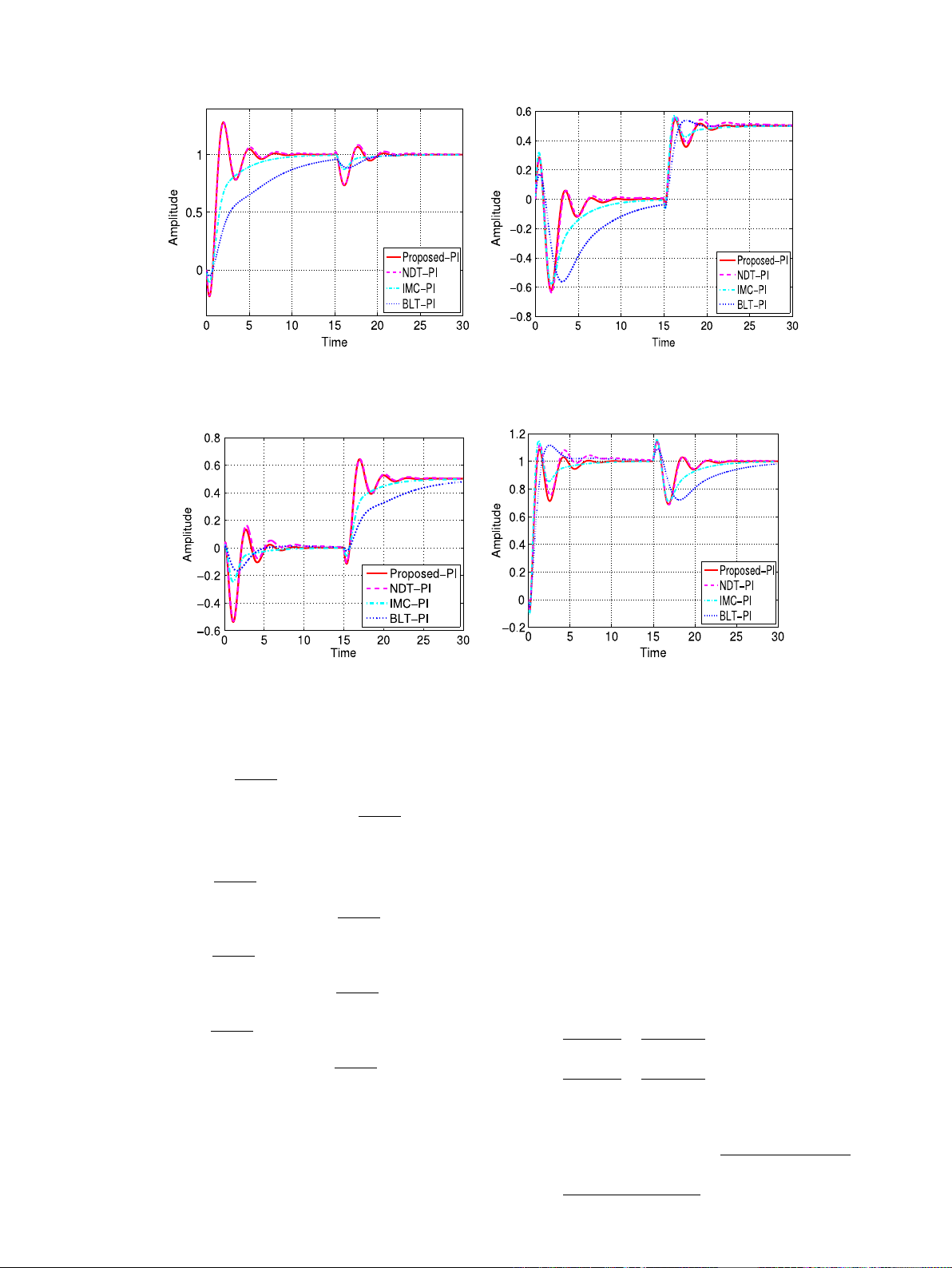
(a) First output to a unit step in the first input. (b) Second output to a unit step in the first input.
Fig. 1. First and second output to a unit step in the first input.
(a) First output to a unit step in the second input. (b) Second output to a unit step in the second input.
Fig. 2. First and second output to a unit step in the second input.
respectively. Using Eqs. (16) and (17), the proposed-PI controller is
KProposed-PI =
−4.0070 −0.6242
s0
0 3.1903 +0.3727
s
.
The NDT-PI, IMC-PI and BLT-PI controllers are given as follows
KNDT-PI =
−3.7960 −0.6671
s0
0 1.8250 +0.2137
s
,
KIMC-PI =
−2.1210 −0.3030
s0
0 3.9510 +0.4295
s
,
KBLT-PI =
−1.0700 −0.1507
s0
0 1.9700 +0.7636
s
.
First and second outputs of resultant control system to unit set-
point change in first input at t=0 and set-point change in sec-
ond input of 0.5 for 16 ≤t≤30 are shown in Fig. 1. Also first
and second outputs of resultant control system to unit set-point
change in second input at t=0 and set-point change in first in-
put of 0.5 for 16 ≤t≤30 are shown in Fig. 2. The performance
indexes such as integral absolute error (IAE), integral square error
(ISE), integral time absolute error (ITAE), peak overshoot (MP)and
rise time (TR)are given in Table 1. From Figs. 1 and 2, and Table 1,
the performance of proposed-PI controller is superior compared to
IMC-PI and BLT-PI controllers. The IAE of proposed-PI controller is
less than NDT-PI, IMC-PI and BLT-PI controllers. The NDT-PI con-
troller is designed by considering gain margin and phase margin
as the robustness constraints. For proposed-PI and NDT-PI con-
trollers, gain and phase margins are calculated. The comparative
results are given in Table 2.
5.2. Example 2
The Wood–Berry binary distillation column process is typi-
cal TITO process with strong interaction and significant time de-
lays [46]. The process has the following transfer function matrix
G2(s)=
12.8e−s
16.7s+1
−18.9e−3s
21s+1
6.6e−7s
10.9s+1
−19.4e−3s
14.4s+1
.
The decoupler matrix is computed from Eq. (2) is
D2(s)=
11.477(16.7s+1)e−2s
21s+1
0.3402(14.4s+1)e−4s
10.9s+11
.
554 D.K. Maghade, B.M. Patre / ISA Transactions 51 (2012) 550–558
Table 1
Performance indexes for example 1.
Controller Input (u)–Output (y)IAE ISE IATE MP(%)TR
Proposed-PI u1–y119.0343 13.6271 41.7848 28.30 1.16
u2–y212.8946 06.9341 32.4502 08.40 0.71
NDT-PI u1–y119.7223 13.6709 47.6276 28.10 1.19
u2–y214.1258 06.8471 47.0779 12.10 0.72
IMC-PI u1–y125.1109 15.4962 60.9464 00.60 1.87
u2–y211.7173 06.1198 32.8835 14.70 0.64
BLT-PI u1–y147.9253 26.4344 199.890 00.00 4.62
u2–y213.8729 07.7046 35.0070 11.60 1.01
Table 2
Gain and phase margins for example 1.
Controller Input (u)–Output (y)Amii % Error (Amii) φmii (°)% Error (φmii)
Proposed-PI u1–y13.0000 0.0000 60.0000 0.0000
u2–y23.0000 0.0000 60.0000 0.0000
NDT-PI u1–y13.0784 2.6134 59.2220 1.2967
u2–y23.0456 1.5200 55.3107 7.8156
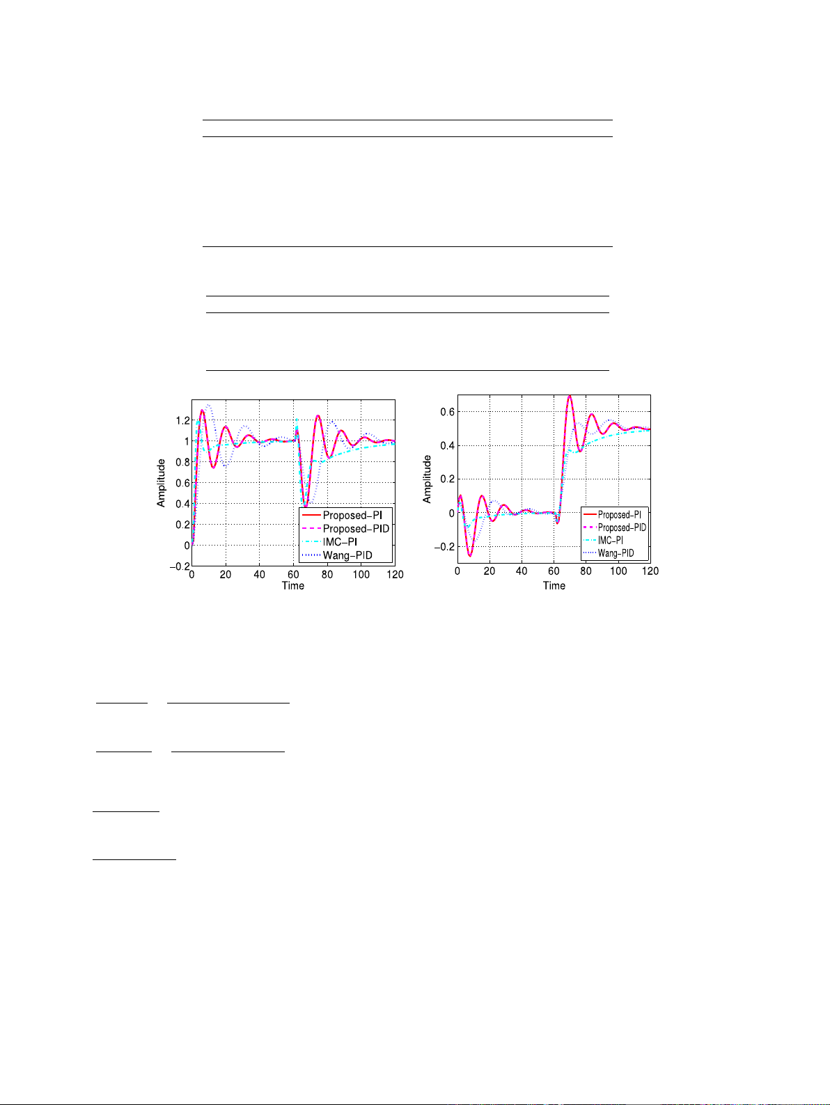
(a) First output to a unit step in the first input. (b) Second output to a unit step in the first input.
Fig. 3. First and second output to a unit step in the first input.
The resulting diagonal subsystems are
h11(s)=12.8e−s
16.7s+1−6.426(14.4s+1)e−7s
(10.9s+1)(21.0s+1),
h22(s)=−19.4e−3s
14.4s+1+9.749(16.4s+1)e−9s
(21s+1)(10.9s+1).
Using Eq. (8), the FOPDT models l11(s)and l22(s)obtained as below
l11(s)=6.37e−0.9335s
5.525s+1,
l22(s)=−9.655e−1.7823s
5.1520s+1.
Using Eqs. (16),(17) and (22), the proposed-PI and proposed-PID
controllers are as given in Box I.
For comparison purpose, two prevalent tuning methods such as
the IMC tuning method and Wang et al.’s auto-tuning method are
applied to G2(s), results in controllers given in Box II.
The IMC method do not use any decoupling method. In this ex-
ample, proposed and Wang et al.’s methods use same decouplers.
For proposed-PI decentralized controller, there are only four tun-
ing parameters, whereas, the Wang-PID controllers have to tune
six parameters.
The step responses of the resultant control system to unit set-
point changes in the first and second inputs are shown in Figs. 3 and
4. The different performance indexes, peak overshoot and rise time
are given in Table 3. Referring to Figs. 3–4and Table 3 proposed-
PID controller results better performance as compared to IMC-PI
and Wang-PID controllers in all respect.
For proposed-PI, proposed-PID and Wang-PID controllers, gain
and phase margins are calculated. The comparative results are
given in Table 4.
6. Real time application
To show the practical applicability, the decoupling method
presented in Section 2and controller design method pre-
sented in Section 4have been tested on laboratory process. A
Level–Temperature reactor process is shown in Fig. 5. The experi-
mental set-up consist of tank with heater. The process is interfaced
to personal computer through data acquisition cards and Emerson
Delta-V DCS software is used to implement the controller. The first
input is an inflow rate through solenoid valve and second input is
power control unit to heater. The first output is liquid level and
second output is liquid temperature in the reactor tank.
For the Level–Temperature reactor the parametric model is
obtained by exciting the system dynamics using PRBS (pseudo-
random-binary-sequence) input. There are numerous types of
input sequences which can provide useful information about
the process, the input is usually changed according to a PRBS
pattern [47]. A PRBS is added to the inputs of process and its effects


![Giáo trình Thực hành Truyền động điện Trường Đại học Bà Rịa - Vũng Tàu [Mới nhất]](https://cdn.tailieu.vn/images/document/thumbnail/2026/20260310/hoaphuong0906/135x160/11121773283865.jpg)
![Giáo trình Thực hành SCADA Trường Đại học Bà Rịa - Vũng Tàu [Mới nhất]](https://cdn.tailieu.vn/images/document/thumbnail/2026/20260310/hoaphuong0906/135x160/94061773283866.jpg)
![Tài liệu học tập La bàn từ [mô tả/định tính]](https://cdn.tailieu.vn/images/document/thumbnail/2026/20260310/hoaphuong0906/135x160/25191773287376.jpg)

![Tài liệu học tập Thiết kế hệ thống nhúng [mới nhất, đầy đủ]](https://cdn.tailieu.vn/images/document/thumbnail/2026/20260305/hoatulip2026/135x160/37051773135929.jpg)


![Giáo trình Điều khiển khí nén thuỷ lực Phần 2: [Mô tả/Chủ đề cụ thể của phần 2]](https://cdn.tailieu.vn/images/document/thumbnail/2026/20260302/camtucau2026/135x160/11911772768225.jpg)
![Giáo trình Điều khiển khí nén thuỷ lực Phần 1: [Mô tả/Định tính thêm nếu cần]](https://cdn.tailieu.vn/images/document/thumbnail/2026/20260302/camtucau2026/135x160/51511772768225.jpg)
![Giáo trình Điều khiển số Phần 2: [Thêm từ khóa mô tả nội dung chương trình]](https://cdn.tailieu.vn/images/document/thumbnail/2026/20260302/camtucau2026/135x160/37201772766913.jpg)
