Automatica,
Vol. 9, pp. 201-207. Pergamon Press, 1973. Printed in Great Britain.
The Design of Linear Multivariable Systems*
La Conception de Syst~mes Lin6aires Multivariables
Der Entwurf linearer multivariabler Systeme
KOHCTpyKLIH~ 0II4HeHHbIX MHOrOBapHaHTHbIX CHCTeM
DAVID Q. MAYNEt
A satisfactory closed-loop linear system may be obtained via a sequence of single-loop
designs, in which classical techniques such as Nyquist diagrams, root-loci etc. are
employed.
Summary--This paper describes a computer-aided procedure
whereby a succession of single-loop designs, using Nyquist
loci, yields a multivariable design which is stable and
attenuates disturbances. The procedure permits more free-
dom than previously available for the selection of the
compensating matrix. It is shown how a simple modification
of the procedure enables security against component failure
to be obtained.
1. INTRODUCTION
THE classical frequency methods for designing
single-loop control systems have proved to be so
useful that it is surprising that so little effort has
been devoted to extending these techniques to
multivariable systems. This may be due to the
development of modern control theory, which
though originally motivated by open-loop trajec-
tory optimisation problems, yielded useful and ele-
gant results for linear multivariable control and
filtering problems. The resultant controllers are
complex, however, requiring a dynamic filter or
observer of almost the same order of complexity as
the plant or process being controlled. In order to
reduce complexity of the controller, CUMMING
[1]
developed a useful algorithm for optimising the
parameters of a given control structure.
ROSmqBROCK, in a pioneering paper [2], redirected
attention to the problem of extending classical pro-
cedures to multivariable problems. Besides pro-
viding a useful theoretical basis, Rosenbrock
* Received 27 March 1972; revised 18 September 1972.
The original version of this paper was presented at the 5th
IFAC Congress which was held in Paris, France during
June 1972. It was recommended for publication in revised
form by Associate Editor H. Kwakernaak.
t Department of Computing and Control, Imperial
College of Science and Technology, Exhibition Road,
London, S.W.7.
describes a useful technique, based on the inverse
Nyquist array, for designing multivariable systems,
and a similar technique using the Nyquist array, and
these methods are extended by MACFARLANE [3].
A series compensator
Go(s)
is chosen to transform
the transfer function
Gp(s),
which is the m x m
matrix transfer function of the system being con-
trolled to
G(s)AGp(s)Gc(s)
where
G(s)
is "diagon-
ally dominant" [2]. Then, m single-loop control
problems are considered, choosing
ks(s), i= 1...m
so that I1
+g~l(j~o)k,(jo~)ll
is large for to < to~ where
is the desired bandwidth for the ith loop and
03 c
the Nyquist "set" consisting of the union of circles
with centre 1
+g,(j~o)k~(jo~)
and radius
E [g'J(Jm)ki(j°~)[)
j=l
j~i
does not encircle the origin. Satisfaction of the
latter condition is a sufficient condition of asymp-
totic stability, and necessary and sufficient if the
system is diagonally dominant in the sense that if
the Nyquist set encircles the origin, completely, the
system is unstable.
The design criteria [3] are assumed to be: (i) per-
formance, e.g. elements of T-l(fio) have small
magnitude for specified range of m--see below, (ii)
stability, (iii) security, or integrity, the maintenance
of stability in face of component failure, and (iv)
low interaction. Stability and performance are
basic criteria. Security is achieved in practice by a
variety of means, e.g. switching to alternative con-
trollers should any component fail, and may have
to be achieved at the expense of performance.
Hence a design method, which ensures stability in
201
202 DAVID Q. MAYNE
the event of the failure of any specified combina-
tions of N components, should also be flexible
enough to include the case N=0. Interaction at
low frequencies is automatically reduced in high
performance systems, and may not be important at
high frequencies, so that, like security, it may not
be an important factor in some designs. Hence, in
the sequel, a basic design algorithm, consisting of a
sequence of single-loop designs, for achieving good
performance and stability is first described. It is
then shown how the algorithm may be modified to
achieve security and, high-frequency, low inter-
action. Diagonal dominance is not necessarily re-
quired, though it can be employed if desired; so
that increased flexibility in the choice of the com-
pensating matrix
Gc(S)
is available. Diagonal
dominance, however, automatically provides se-
curity against arbitrary, output transducer failure
and also limits interaction.
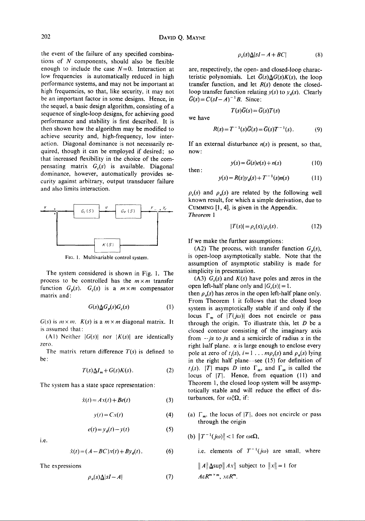
K(S)
FIG. 1. Multivariable control system.
The system considered is shown in Fig. 1. The
process to be controlled has the m xm transfer
function
Gp(s). Gc(s )
is a
m×m
compensator
matrix and:
G(s) AGp(S)Gc(S)
(1)
G(s)
is m x m.
K(s)
is a m x m diagonal matrix. It
is assumed that:
(A1) Neither IG(s)l nor IK(s)] are identically
zero.
The matrix return difference
T(s)
is defined to
be:
r(s)Alm + G(s)K(s).
(2)
The system has a state space representation:
2(t) = Ax(t) + Be(t)
(3)
pc(s)Alsl- A + BC[
(8)
are, respectively, the open- and closed-loop charac-
teristic polynomials. Let
G(s)A_.G(s)K(s),
the loop
transfer function, and let
R(s)
denote the closed-
loop transfer function relating
y(s)
to
Yd(S).
Clearly
G(s) = C(sI- A)- 1B.
Since:
T(s)G(s) = G(s)T(s)
we have
R(s) = T- I(s)G(s) = G(s)T- l(s).
(9)
If an external disturbance
n(s)
is present, so that,
now:
y(s) = G(s)e(s) + n(s)
(10)
then :
y(s) = R(s)ya(s) + T- 1 (s)n(s) (11 )
pc(s)
and
po(s)
are related by the following well
known result, for which a simple derivation, due to
CUMMING [l, 4], is given in the Appendix.
Theorem 1
IT(s)[ =
pc(s)/pc(s).
(12)
If we make the further assumptions:
(A2) The process, with transfer function Gp(s),
is open-loop asymptotically stable. Note that the
assumption of asymptotic stability is made for
simplicity in presentation.
(A3)
Go(s)
and
K(s)
have poles and zeros in the
open left-half plane only and ]Gc(s)[ = 1.
then
po(s)
has zeros in the open left-half plane only.
From Theorem 1 it follows that the closed loop
system is asymptotically stable if and only if the
locus F,, of ]T(jog)l does not encircle or pass
through the origin. To illustrate this, let D be a
closed contour consisting of the imaginary axis
from --j~ to j7 and a semicircle of radius ~ in the
right half plane. ~ is large enough to enclose every
pole at zero of
ti(s), i= 1 ... mpc(s)
and
po(s)
lying
in the right half plane--see (15) for definition of
t~(s).
ITI maps D into F m, and F,, is called the
locus of ITt. Hence, from equation (11) and
Theorem t, the closed loop system will be assymp-
totically stable and will reduce the effect of dis-
turbances, for ~o~fL if:
i.e.
y(t) = Cx(t) (4)
e(t)
= yd(t)-y(t) (5)
2(t) = ( A - BC)x(t) + Byd(t).
(6)
(a) F,., the locus of IT[, does not encircle or pass
through the origin
(b)
IIT-'(J )II <
1 for ogefL
i.e. elements of
T-~(jog)
are small, where
The expressions
po(s) AlsI- A[
(7)
II AH~sup]l Axll subject to !IxN = 1 for
AeR" "", xeR".
The design of linear multivariable systems 203
To achieve (a) a single-loop design is often satis-
factory. To achieve (b) m "tight", or high gain,
loops are required. These can be designed sequen-
tially. For convenience some extra terms, appro-
priate to the condition when the first i loops are
closed and the remaining open, i.e.
kj(s)=O,
j = i + 1 ... m,
are defined:
K,(s)A_diag(kt(s), ...
k,(s), 0... 0) (13)
Note:
T~(s)AI= + G ° "(s)Ki(s)
(18)
G'" "(s)A[T~(s)]-'G °, "(s)
(19)
ff(s)A l -- k ",s" i - 1
+ il.')gii ' "(s).
(20)
6 °. ~(s) = C,°(s) = 6(s).
T i(s)AIm + G(s)K i(s)
(14)
Gi(s)A Ti '(s)G(s)
(15)
for i= 0... m. Clearly
To(s) =Ira, G°(s) = q(s).
G~(s)
is the transfer function relating y to v (Fig. 1)
when loops i+ 1 ... m are open. We also define,
for i= 1 ... m, the scalar return difference:
ti(s)A_
1 +
ki(s)giF
1 (s)
where
gkj(s)
is the/jth element of
Gk(s).
(16)
It is shown below that if the scalar return dif-
ferences t~(s), where t i maps D into ~i, the locus of
t, i= 1... m can be chosen to satisfy the usual
criteria, i.e. magnitude of
t,(fio)
is large for coef~ and
7~ does not encircle or pass through the origin,
then the resultant closed loop system is satisfactory
in the sense of satisfying (a) and (b) above. Hence
a naive design procedure, currently used in practice,
would be to choose k~ so that t~ = 1
q-k~g~t
is satis-
factory, calculate G 1, choose k z so that
t 2 = 1 + kzg~22
is satisfactory, calculate G z etc. However this pro-
cedure ignores the fact that even if
]Gp(S)[
has no
right-half plane zeros, so that m tight loops are
possible [5], g171, i= 1 ... m, as obtained above,
may have right-half plane zeroes. The role of Go
where
IG~(s)[
= 1, in the
basic
algorithm, which has
the objectives: performance and asymptotic stabi-
lity, is to ensure that, if possible, g~7 ~, i= 1... m
have no right half plane zeroes and to apportion
"design difficulty" appropriately to the various
loops.
As shown below the above procedure achieves
security for the following fault conditions:
simul-
taneous
failure of, output, transducers j, j+ 1... m
(or,
kj=ki+l
.... k,,=0) for j=l ... m. Note
that if G=
G~Gp
rather than G=
GpG~,
the system
is secure against simultaneous failure of input,
actuators, j, j+ 1 ... m (or
kj=kj+ 1
.... km=0)
for j= 1 ... m. In other cases the transfer functions
G~(s),
~=2... N corresponding to each fault, i.e.
G~(s)AA.Gp(s),
must be calculated. For a=l... N,
i=0.., m we define:
G °' ~(s)AG~(s) Gc(s)
(17)
For i=l...m, k ~ is chosen so that the N loci
y~', a= 1... N, where tf maps D into y~, are satis-
factory. This achieves security, but places an extra
requirement on k~, possibly leading to a reduction
in performance,
unless
these loci are close together.
For the case of arbitrary transducer failure, i.e.
actuator failure if G =
GcGp,
this can be achieved by
choosing Gc so that G is diagonally dominant
or
so
that G is approximately upper or lower triangular,
i.e.
g~j-O
for allj<i or for ailj>i. For mixed
transducer, actuator failure, there does not neces-
sarily exist a G~ such that the loci y~, ~= 1 ... N
are close together, so that a reduction in per-
formance may result.
It is shown below that if the loop gains are high
for ogef2, the closed loop transfer function
R(jo~)--,L
so that interaction is low. At high fre-
quencies,
R(flo)~G(jto),
so that low interaction at
high frequencies, if considered important, can be
achieved by choosing G c so that
G(jco)
is approxi-
mately diagonal as co~.
The design procedure commences by relabelling
inputs and outputs, which corresponds to pre- and
post-multiplication by permutation matrices, so
that the resultant Gp is preferable, i.e. if possible.
[Gp(0)] u > [Gp(0)]~j for all j# i.
Justification for the above comments and for the
design algorithm follow from the results given in
§2. The algorithm is specified in §3.
2. BASIC RESULTS
Let gi., g.i denote, respectively, the ith row and
the ith column of G. Let
So
denote the open-loop
state space representation (A, B, C) of
a~(S) ac(S)K(s)
given in equations (3) and (4). Let S,, denote the
closed-loop state space representation
(A-BC,
B, C) given in equations (3), (4) and (5). For
i= l... m, let S i denote the state space representa-
tion
(A-BIC , Bi, C)
corresponding to the situation
when the first i loops are closed and the remaining
are open, i.e.
kj(s)-O, j=i+l...m.
Let
p~(s)
=]sI-A+B,C[
denote the characteristic poly-
nomial of S~. ~i, resp. F~, is the locus of ti, resp.
]Til, i.e. t~ maps D into ~'i etc.
204 DAVID Q. MAYNE
The first result, also proven independently by
ROSENBROCK
[6], is:
Theorem 2
For i=l ... m
I T,(s)l-- FI
tj(s).
(21)
j=l
Proof
I To(s)[ = 1
I T,(s) I -- IT,_ ,(s)
+ k,(s)g.(s)e[[
= I T,_,(s)[]I,,,+ k,(s)g'?'(s))e~[
= I T, _, (s)[(1
+
k,(s)g~7-'
(s))
=
IT,_, (s)]t,(s).
(22)
The result follows by induction.
A direct corollary of this result is the following
stability theorem, which also proves the assertion
in §l about security in face of simultaneous failure
of, output, transducers j+ 1 ... m, for j= 1 ... m.
Theorem 3
Let
A~-A 3
be satisfied. If Yl • • • 7,, each satisfy
the Nyquist criterion, i.e. 7, does not encircle or
pass through the origin, i= 1 ... m, then
$1 • • •Sm
are asymptotically stable.
Proof.
Let
p*~(s)
denote the characteristic poly-
nomial of
Si,
i.e. p~ has the same degree n as
po, p~.
From Theorem 1 :
I T,(s)[ =
p~(s)/Po(S).
(23)
Let N~, n, denote, respectively, the number of net
encirclements of the origin by F~ and y~. From
Theorem 2:
i
Ni = Z nj.
(24)
j=l
Since
po(S)
has no right half plane roots, N~ is
equal to the number of roots of
p~(s)
in the right
half plane. The result follows.
The next result gives a simple sequential method
for calculating G i and q, i= 1... m.
Theorem 4
The following algorithm generates G', h,
i=1 ...m:
(i) Set
Gi(s)=G(s).
Set i= 1.
(ii) Set t,(s) = 1 + k;(s)gl/- ~(s).
(iii) If i= m, stop. Otherwise:
Set
~i(s)=ki(s)/t,(s)
(25)
G i- 1 s ~ s _i- l/sX_i-
Set Gi(s)= ( )- "i( )v., t mi. 1(s) (26)
Set i= i+ 1.
(iv) Go to (ii).
Proof.
Ti(s) =
Ti- l(s) + ki(s)o.,(s)eT
= T,_ ~(s)[l,, +
k,(s)g!; ~(s)er].
(27)
Hence, using a well known identity to invert the
term in brackets:
T F ~(s)G(s) = [I,,- Fg(s)917 '(s)eT]G '- t(s) .
The result follows.
The next result shows how "tight" loops reduce
G'=TF~G,
and hence, since
Ia(s)l 0, TF',
i=l...m.
Theorem 5
(a) Let
ti(s)=~i(s),
i=1.., m, where the co-
efficients of the rational function a t are finite
and
ai(s)~O.
Then, for i= 1 ... m:
i
rAi(s)
F'(s)/~-] .
_i,,
.,(s) j+,,s,
where
Ai(s) = diag(91
l(s)/q(s) . . . 917 l(s)/h(s))
and the coefficients of the elements of U are
fo order 1/~2 and L{ a = 0 if p >1 i and q t> i.
(b) If
G°(s)
is lower, resp. upper, triangular, then
Gi(s)
is lower, resp. upper, triangular,
i=1 ...m.
Proof.
(a) From Theorem 4,
9!i
and Ol. are give
by:
oi,(s)
=
g!F
1(00 -
~,(s)olF'(s))
= 9!7 X(s)/ti(s)
(29)
i S i-
9i.( ) =0z. 1(0(1 -
~i(s)oi[l(s))
= oiT'(s)/t,(s)
(30)
i.e. the ith loop reduces the ith yow and ith column
of
G i-1
by a factor
1/ti.
Suppose
G i-l(s)
has the
form given in equation (28), with i replaced by i- 1.
Application of equations (26), (29) and (30) show
that G i then has the form of equation (28). Since
G has this form, using equations (29) and (30), the
result follows.
(b) The result follows from equation (26).
Note that
Gm(s)--.O
as c~--.~, and
R(s)
= GmK(S)~I.
Result (b) merely states the well known fact that
control loops for lower, or upper, triangular systems
can be independently designed.
The design of linear multivariable systems 205
The final result gives an estimate for 0171(s) if
loops 1... i--1 are "tight", i.e. ~t~oo; see also,
ROSEYaROCK [5], where this result first appears. Let
[A]kdenote the k x k matrix whose
pqth
element is
dpq.
Let
Ak(s)Al[G(s)kl.
Theorem 6
For i= 1... m:
= ds) +
(v) Choose
G~+l(s). (GT(s)=I,,):
Set
G i' ~(s) = G i' ~(s)Gi, + t(s), ~ = 1 . . . N.
Set i=i+ 1.
(vi) Go to (ii).
Comment
I. The final compensation matrix is:
G~(s) = Gt~(s). G~(s) . . . GT(s ) .
where Ao(s)A1, and 0(1/0t) denotes a rational poly-
nomial function, whose coefficients are of order
1/ct.
Proof
From equation (26), for k_> i
[G/(s)]k =
[Im --
li,(s)o.,(s)eTJ,[G'-'(s)]~.
Let
A~(s)A[G'(S)]k.
Hence, fork>i; i=l...m:
Hence
A~(s) = A~-
'(s)/t,(s).
(31)
Aj- t(s) = Aj(s)//_~ ~
q(s).
(32)
But from Theorem 5:
j--I
Aj-'(s) = g~f '(s) I] [giT'(s) + O(1/a)]/ti(s). (33)
i=1
The result follows directly.
3. THE DESIGN ALGORITHM
For i= 1 ... m, let
G~(s)
denote a compensating
matrix, representing a sequence of elementary
(column) operators, so that
[Gic(s)l
= 1, having the
structure:
o]
Algorithm
(i) Recorder inputs and outputs as required
Because of the structure of G~, i= 1 ... m
.
.
T~(s)AI,,, + G~,(s)Gc(s)Ki(s)
= I,, + G~,(s)[GIc(s)... G*~(s)]Ki(s)
so that T7 is unaffected by
G~, j>i.
It is
easily deduced that the theorems of §2 are
unaffected by this sequential choice of G~.
If an approximate lower triangular system is
required,
G~'l(s)
must be chosen so that
#1]t't(jco)-0, j=i+l .... m, for all ogel].
If an approximate diagonal system is required,
in addition to the above,
G~(s)
must be chosen
so that
G°'~(jog)
is approximately upper
triangular.
In addition
G~(s)
must be chosen so that, if
possible, g~7 t, 1(0 is minimum phase,
i=l...m-1.
. Since [G~(s)[ ~ 1, it follows from Theorem 6,
that, if m high-gain loops are possible, i.e.
[Gp(s)[ is minimum phase, then:
of,-" '(s)= I G,,(s)l + 00/ )
i=1
so that G,, in effect, shares the magnitude and
phase characteristics of
G~(jo~)
between the
various loops.
Note that if
IGp(s)l
has right half zeros,
these zeros will appear in one or more loops
if the remaining loops are tight.
(ii) Choose
G~(s).
Set
G °'
~(s)=
G~,(s)G~(s), ~= 1 ... N.
Set i= 1.
(iii) Set
t~(s)=l k's" i-1
~"s"
+ i()gu ~),~=I...N.
Choose
ki(s ).
(iv) If i=m, stop. Otherwise, for ~= 1 ... N
Set/c~(s) =
ki(s)/t~(s).
Set G" ~(s) =
G i- 1. ~(s) - l¢~(s)g~; t, ~(s)glf l, ~(s).
.
.
ki(s)
is chosen so that the Nyquist loci
?T, ct = 1.. N, do not encircle the origin, and,
if possible,
I#(jco)l
>> 1 for coef~.
If the resultant system is not satisfactory,
K(s)
can be altered by repeating the design
procedure with G o, ~(s) set equal to Gm' ~(s)
of the first iteration, ~= 1... N, (which is
approximately diagonal if m high loop gains
were achieved in the first iteration) and
Go(s)
left unaltered. However the designer will now.
"see" G ''~ which differs appreciably from
G O, ~, the original system with compensation.


![Bài giảng Vi điều khiển Nguyễn Huy Hoàng: Tổng hợp kiến thức [Chuẩn nhất]](https://cdn.tailieu.vn/images/document/thumbnail/2026/20260316/hoatrami2026/135x160/72211773806757.jpg)


![Bài giảng Tự động hoá thiết bị điện [chuẩn nhất]](https://cdn.tailieu.vn/images/document/thumbnail/2026/20260312/hoabattu2026/135x160/61691773631881.jpg)
