Automatica,
Vol. 12, pp. 211-224. Pergamon Press, 1976. Printed in Great Britain
The Design of a Multivariable Control
System for a Ship Boiler*
ARNE TYSS~,? J. CHR. BREMBO~ and KJELL LIND§
An application of linear regulator theory in the design of multivariable control
systems/or nonlinear processes
Summary--A multivariable control system is designed for a
large scale ship boiler. The design is based on concepts of
modern control theory and extensive use of all-digital
real-time simulation.
This paper describes in particular how it is possible to
verify the multivariable control system without having the
real process operating.
1. INTRODUCTION
THE SOtLER studied in this paper is a Foster
Wheeler ESD III with a normal steam production
of 21.9 kg/sec. The boiler is operated on the basis
of natural circulation. The control system is
designed to maintain the drum level, drum
pressure and the steam temperature at pre-
scribed reference values given by the load
condition. A Kalman filter for the estimation of
the process state as well as the environmental
state vector is included. The environment is
supposed to produce slowly varying distur-
bances to the process.
The integral control action (reset) is provided
by an external decoupled integrator loop, and the
integral action in the estimation loop follows
from the assumptions about the disturbance
model.
The external integrator structure also gives a
simple solution to the 'bumpless transfer' prob-
lem, that is a soft transfer from conventional
back up system mode to multivariable mode.
By means of simulation facilities it is possible
to examine the behaviour of the control system
for all kinds of manoeuvres and disturbances.
Examples of such tests will be presented.
*Received August 14, 1975; revised May 19, 1975; revised
December 2, 1975. The original version of this paper was
presented at the IFAC/IFIP Symposium on Ship-Operation-
Automation which was held in Oslo, Norway during July
1973. The published Proceedings of this IFAC Meeting may
be ordered from: IFAC/IFIP Conference, Gloriastrasse 35,
CH-8006, Zurich. This paper was recommended for publica-
tion
in revised form by associate editor K. J. ~strfm.
?The
University of Trondheim, The Norwegian Institute of
Technology, Division of Engineering Cybernetics.
~The Ship Research Institute of Norway, Trondheim,
Norway.
§Sonnico Pan Electric Contracting A/S, Oslo, Norway.
The integrity of the control system will be
discussed, and the digital real time simulation
system which consists of two process control
type computers, will be described in some detail.
Important works in the field of boiler models
and boiler control systems are given by
Eldund[5], Anderson[16], Kwan and Ander-
son[19], Nicholson[17], [18], Waiters and
Williams[20], McDonald and Kwatny [21],
McDonald, Kwatny and Spaare [22].
The paper is divided into two parts:
1. The theoretical work necessary for the
control system's design.
2. The application of the all digital real time
simulation in evaluating the control system.
2. THEORETICAL WORK
2.1
The boiler model
The original nonlinear dynamic model was of
twentieth order[l]. It was assumed to consist of
lumped energy storage elements comprising
steam drum, downcomers, mud drum, risers,
primary and secondary superheater, desuperhea-
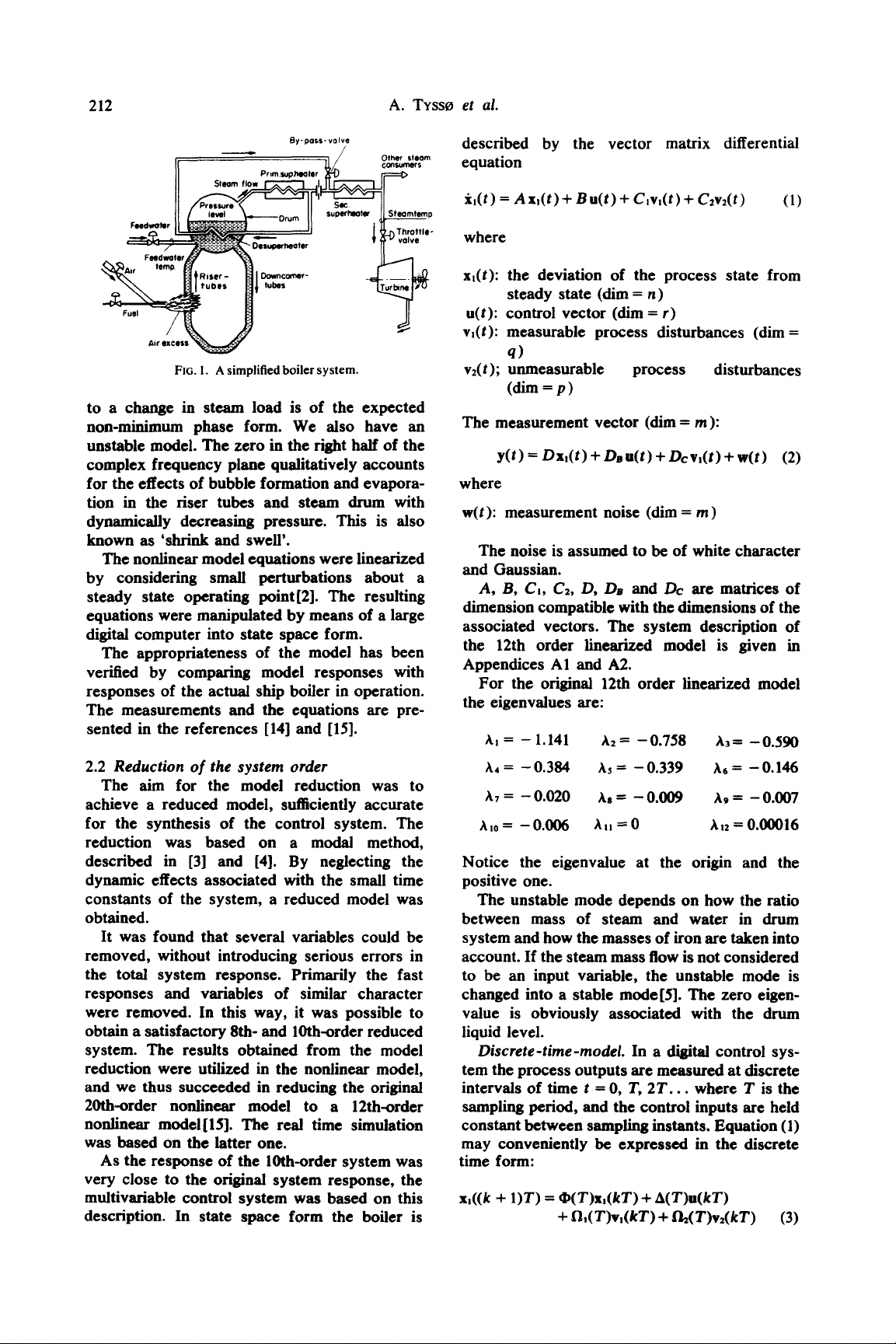
ter and economiser. Figure 1 shows a simplified
boiler system. The mathematical model was
designed basically for the two following pur-
poses.
(a) To be a basis for a linearized model to be
used for design of the multivariable control
system.
(b) To study the multivariable control system
by means of real time simulation.
For purpose (a) it is desirable to reduce the
model to the lowest possible order. This is to
keep the computing time and storage at a
minimum, and to r,educe the number of state
variables to influence the control system's
design. It has been shown that the optimal
controller can be of rather simple form.
For purpose Co) it is desirable to have a
nonlinear model which accurately describes the
actual boiler system.
The simulated model responses are mostly of
simple form, but the response of the drum level
211
212 A. TYsso
et al.
By-pass-valve
/ "
Feedwoter
'
_ I~;C~
II |
',,Th,o*.e-
Feedwater ~:.I '~,_~
Air
temp. ~ -
_. ;-
FIG. I. A simplified boiler system.
to a change in steam load is of the expected
non-minimum phase form. We also have an
unstable model. The zero in the right half of the
complex frequency plane qualitatively accounts
for the effects of bubble formation and evapora-
tion in the riser tubes and steam drum with
dynamically decreasing pressure. This is also
known as 'shrink and swell'.
The nonlinear model equations were linearized
by considering small perturbations about a
steady state operating point[2]. The resulting
equations were manipulated by means of a large
digital computer into state space form.
The appropriateness of the model has been
verified by comparing model responses with
responses of the actual ship boiler in operation.
The measurements and the equations are pre-
sented in the references [14] and [15].
2.2
Reduction of the system order
The aim for the model reduction was to
achieve a reduced model, sufficiently accurate
for the synthesis of the control system. The
reduction was based on a modal method,
described in [31 and [4]. By neglecting the
dynamic effects associated with the small time
constants of the system, a reduced model was
obtained.
It was found that several variables could be
removed, without introducing serious errors in
the total system response. Primarily the fast
responses and variables of similar character
were removed. In this way, it was possible to
obtain a satisfactory 8th- and 10th-order reduced
system. The results obtained from the model
reduction were utilized in the nonlinear model,
and we thus succeeded in reducing the original
20th-order nonfinear model to a 12th-order
nonlinear model[15]. The real time simulation
was based on the latter one.
As the response of the 10th-order system was
very close to the original system response, the
multivariable control system was based on this
description. In state space form the boiler is
described by the vector matrix differential
equation
i,(t)=Ax,(t)+Bu(t)+C,v,(t)+C2v2(t)
(1)
where
x,(t): the deviation of the process state from
steady state (dim = n)
u(t): control vector (dim = r)
v,(t): measurable process disturbances (dim=
q)
V2(t),
unmeasurable process disturbances
(dim = p)
The measurement vector (dim = m):
y(t)=Dx2(t)+DBu(t)+Dcvt(t)+w(t) (2)
where
w(t):
measurement noise (dim = m)
The noise is assumed to be of white character
and Gaussian.
A, B, C,, C2, D,/)8 and
Dc are
matrices of
dimension compatible with the dimensions of the
associated vectors. The system description of
the 12th order linearized model is given in
Appendices A1 and A2.
For the original 12th order linearized model
the eigenvalues are:
Ai = -- 1.141 ,t2 = --0.758 a3= --0.590
A4 = --0.384 A5 -- --0.339 ?,6= --0.146
;t7 = - 0.020
As
= - 0.009 ~,9 = - 0.007
Ai0 = --0.006 All =0 An = 0.00016
Notice the eigenvalue at the origin and the
positive one.
The unstable mode depends on how the ratio
between mass of steam and water in drum
system and how the masses of iron are taken into
account. If the steam mass flow is not considered
to be an input variable, the unstable mode is
changed into a stable model5]. The zero eigen-
value is obviously associated with the drum
liquid level.
Discrete-time-model.
In a digital control sys-
tem the process outputs are measured at discrete
intervals of time
t = 0, T,
2T... where T is the
sampling period, and the control inputs are held
constant between sampling instants. Equation (1)
may conveniently be expressed in the discrete
time form:
x,((k + 1)T) =
~(T)x,(kT) + A(T)u(kT)
+ fl,(T)v,(kT) + l'h(T)v2(kT)
(3)
The design of a multivariable control system for a ship boiler 213
The choice of sampling rate depends on the
process and valves dynamics and the noise
characteristics.
By removing the two fastest eigenvalues from
the 12th-order model the fastest eigenvalue in the
new 10th order model is given by ?,3 ffi -0.59.
This indicates theoretically a sampling rate not
lower than 0.9 sec. Simulations, however, have
shown that a sampling rate T ffi 2 sec is sufficient.
The 10th order model is given in Appendix A3.
2.3
Control philosophy
The optimal control with state variable feed-
back is determined from the minimization of the
quadratic objective functional given a unit
sampling interval
J = 2(x(N) - x~)Ts (x(N) - x~)
N--I
(4)
where x~ is the desired state. S and Q are
positive, semideflnite symmetric, constant mat-
rices which penalize the final state offsets and the
deviation in the state variables, respectively. P is
a symmetric matrix of constants which penalize
use of control action and must be positive
definite.
The solution of this problem can be separated
into two independent problems
(a) a deterministic control problem.
Co) an estimation problem.
The deterministic control strategy is known to
be
u(k) - Gx,(k)
= - P-' A T~P-T(R (k )
-
Q)x,(k)
(5)
It is difficult
a priori
to choose the parameters
in the loss functional. As a rule of thumb we use
i= l,2,...,n
j--1,2 ..... r
as initial guess of Q and P. Through a simulation
it is possible to see if the feedback controller is
satisfactory. The constraints and dynamic limita-
tions in the control variables are not taken into
account explicitly. Therefore we have to balance
a fast response against a realistic magnitude of
the control variables. The final answer to this
question will be given by the real time simulation
in the data laboratory. It is important that the
feedforward terms, discussed below, are in-
cluded in the simulation.
To implement an optimal control it is neces-
sary that every element in the state vector be
available for measurement. In our case only two
components of the state vector are measured
directly, so it is necessary to estimate the others.
The estimator is based on a reduced, linear
model of the process. The solution will therefore
be sub-optimal.
It is known that the least squares estimator is
described by
il(k
+ 1) = ~,(k) + An(k) + flv,(k)
+ ~K,(y(k) - ~(k))
(8)
where ^ denotes estimates. In equation (8) KI is
given by
K, = AX(k)DT(DAX(k) +
W(k))-' (9)
where
AX(k ) = E(~,(k )Ax,T(k ))
= E ((x,(k) -
i,(k)Xx,(k) - ~,(k)) 'r)
where R is determined from the discrete matrix
Riccati equation
R(k)ffi Q
+~pT(R-'(k +
I)+AP-'AT)-'~ (6)
with boundary condition
R(N) = S (7)
For the boiler application we will use the
stationary value of the feedback matrix
G(k).
The terminal time can be regarded as plus
infinity. This also means that S can be set equal
to zero.
and
W(k) ffi= E(w(k)wr(k))
are the covariance matrices of the state estima-
tion error and the measurement noise, respec-
tively.
AX(k)
can be determined as the solution
of a discrete matrix Riccati equation.
The main objective for the multivariable
controller is to keep three variables at prescribed
reference values given by the load condition.
The prescribed reference vector
r~(k) ffi f(v,(k)) (10)
214 A. Tvsso et al.
The reference variables are:
y, = drum pressure
y~ = steam outlet temperature
y3 = drum level
or expressed in an equation:
where
r(k)
=
Ty(k)
r(k) = reference vector, (dim = 1).
In the stationary state we require:
(11)
both the process and the environment is de-
scribed by
r,,.)1
=LU I U
J
,(t)
L~--~J
+ [-~]v,(t)+ [O]n(t) (17)
and can be written
,(t) = Ax(t)
+/]u(t)+
~v,(t)+ #n(t) (18)
and in the discrete-time form
x((k + I)T) = ~(T)x(kT) + f~(T)u(kT)
+
~(T)v,(RT)
+
O(T)n(RT)
(19)
r(k) - r,a(k) = 0 (12) The gain in the extended estimator is now
2.4 Elimination of steady state errors
If the control law given by equations (5) and
(8) is used without any additional features, there
will be two kinds of stationary errors in the
multivariable control system; one in the estima-
tion loop and one in the control loop.
This is due to the fact that we use an
approximated model in the estimator, and that
the process is influenced by disturbances (equa-
tion 1).
The difference between the actual measure-
ment and the estimated one can be expressed
Lim
{y(t) - S,(t)}
=
Ay (13)
t--~z
The steady state offset error in the control loop
can be expressed
Lim
{r(t) - r~,r(t)}
-- Ar
(14)
f~
In [6] it is shown that this special choice of
dynamics of the environment leads to an integral
action in the estimation loop.
The assumed covariance of the environment
excitation determines the way in which i~(k) will
track x2(k), since K2 determines the reset time
for tracking x2(k) in the estimator. It is always
difficult to assume reasonable values for the
environment excitations, and therefore we have
used a modal method to determine K,. Thus we
specify in advance the desirable reset time in the
estimation loop. It is reasonable to assume that
the process estimator is considerably faster than
the environment estimator. If H is the specified
eigenvalue matrix (with diagonal elements only)
for the environment, we find that
K2 = (I-H)(D(I-O+OK,D)O)-' (20)
The estimation loop. The estimation loop
problem can be solved by regarding the error as a
slowly varying process disturbance and estimate
this in an estimator.
The environment which generates the distur-
bances is described by a Wiener process
i~(t) =Fn(t)
(15)
v,(t) = Hx2(t) (16)
where
x2(t):
environment state vector (dim = 1)
n(t): white noise, zero mean vector.
The state of the "supersystem' encompassing
K, is determined from the equation for optimal
estimation. A necessary condition for (D(I - • +
OK,D)O)-' to exist is that the number of
environmental states is assumed to be equal to
the number of measurements (m ffi p). If m < p,
the environment model is not observable.
The control loop. Depending on whether the
disturbance can be measured or not, we will have
the following solutions:
(a) When the disturbance vector can be
measured directly, a feedforward vector can be
produced from the disturbance vector.
(b) When the disturbance vector cannot be
measured, a control strategy which performs
integral action in the control loop will be used.
If the prescribed reference vector is regarded
as a measurable disturbance, the control law
The design of a multivariable control system for a ship boiler 215
including the feedforward then is: Now let
u(k) =
Gi,(k)+ G,r.~(k)+
G4v,(k) (21)
The feedforward matrices can be determined as
follows:
In the stationary state we have:
i,(k
+
I) = t,(k) (22)
From equation (2) and (11) we then have
r(k) =
T(D + DBG)i,(k ) + TD.G3r..-(k )
+ T(DuG4 + Dc)v,(k)
(23)
G is found from equation (5) and from the
condition r(k)= r,~(k) we have:
G, = ((TD. - T(D + DBG)(O - I +
AG)-'A)-' (24)
G4 = Gs(T(D + DsGX~ - I + AG)~ - TDc)
(25)
A condition for G3 to exist is that T have the
dimension r x m.
The integral action in the control loop is very
important. From a theoretical point of view it is
possible to obtain this in different ways. In [6] it
is proposed to use a feedback from the estimated
environmental state, and in [7] and [8] it is
proposed an external integrator loop by aug-
menting the state vector with an integration
vector (equation 27). It is also possible to obtain
integral action by weighting higher order time
derivatives of u in the performance index.
Regarding a practical implementation of the
integral action, attention must be paid to the
'wind up' problem, which seriously occur when
control variables are temporarily or permanently
in the saturated state.
The implemented solution is based on use of
an external decoupled integrator structure[13]
controlled by a computer program. The number
of integrators must be less or equal the number
of control variables. Thus the process is output
controllable with respect to r if l <- r.
The complete control law will be
z = (28)
and the performance index could now be
1
], = (x(k)- +
o(k)Tpu(k)
+ (r(k) - r,,dk))TQ~(r(k) - r~(k)) (29)
Expressions for the feedback-feedforward
matrices are given in Appendix A4. G2 will now
not be in diagonal form, and will thus only give
the initial values for a final solution.
The weighting elements for the augmented
states must be carefully chosen, so that their
dynamics do not influence the main dynamic
behaviour. This can be examined by studying the
eigenvalues in the closed feedback loop with and
without the integration vector included.
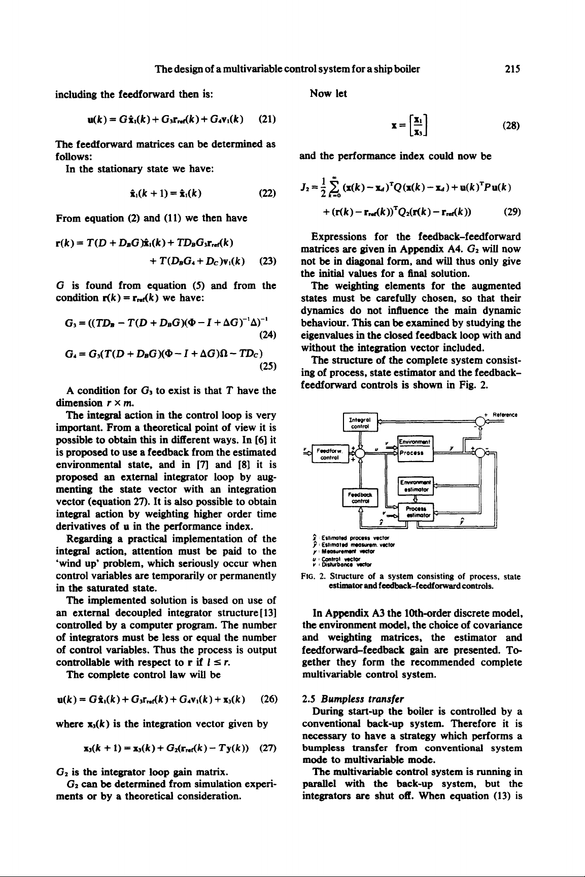
The structure of the complete system consist-
ing of process, state estimator and the feedback-
feedforward controls is shown in Fig. 2.
~: Estimated process vector
: Estimated meosurem vect~'
¥ : Measuremenl vector
u : Control voctor
v , Dislwbonce voct~
+ Reference
FIG. 2. Structure of a system consisting of process, state
estimator and feedback-feedforward controls.
In Appendix A3 the 10th-order discrete model,
the environment model, the choice of covariance
and weighting matrices, the estimator and
feedforward-feedback gain are presented. To-
gether they form the recommended complete
muitivariable control system.
u(k) = G/,(k) + G3r,,,(k) + G,v,(k) + x3(k) (26)
where x3(k) is the integration vector given by
x~(k + 1) = x3(k) + G2(r,.f(k)- Ty(k)) (27)
G2 is the integrator loop gain matrix.
G2 can be determined from simulation experi-
ments or by a theoretical consideration.
2.5
Bumpless transfer
During start-up the boiler is controlled by a
conventional back-up system. Therefore it is
necessary to have a strategy which performs a
bumpless transfer from conventional system
mode to muitivariable mode.
The multivariable control system is running in
parallel with the back-up system, but the
integrators are shut off. When equation (13) is


![Bài giảng Vi điều khiển Nguyễn Huy Hoàng: Tổng hợp kiến thức [Chuẩn nhất]](https://cdn.tailieu.vn/images/document/thumbnail/2026/20260316/hoatrami2026/135x160/72211773806757.jpg)


![Bài giảng Tự động hoá thiết bị điện [chuẩn nhất]](https://cdn.tailieu.vn/images/document/thumbnail/2026/20260312/hoabattu2026/135x160/61691773631881.jpg)
