Bài giảng Tối ưu hóa nâng cao: Chương 10

Newton’s Method

Hoàng Nam Dũng

Khoa Toán - Cơ - Tin học, Đại học Khoa học Tự nhiên, Đại học Quốc gia Hà Nội

Newton-Raphson method

http://www.stat.cmu.edu/~ryantibs/convexopt-F13/ scribes/lec9.pdf

http://mathfaculty.fullerton.edu/mathews/n2003/ Newton’sMethodProof.html

http://web.stanford.edu/class/cme304/docs/ newton-type-methods.pdf

Annimation: http://mathfaculty.fullerton.edu/mathews/a2001/ Animations/RootFinding/NewtonMethod/NewtonMethod.html

Newton’s method

Given unconstrained, smooth convex optimization

f (x), min x

where f is convex, twice differentable, and dom(f ) = Rn. Recall that gradient descent chooses initial x (0) Rn, and repeats ∈

−

1)), −

x (k) = x (k f (x (k k = 1, 2, 3, . . . tk − · ∇

In comparison, Newton’s method repeats

2f (x (k

1)),

−

1)) −

−

(cid:16) (cid:17)− x (k) = x (k f (x (k k = 1, 2, 3, . . . − ∇ ∇

1).

2f (x (k

1)) is the Hessian matrix of f at x (k

−

Here ∇

Newton’s method interpretation

Recall the motivation for gradient descent step at x: we minimize the quadratic approximation

2 2, (cid:107)

y x f (y ) f (x) + f (x)T (y x) + ≈ ∇ − 1 2t (cid:107) −

t over y , and this yields the update x + = x f (x). − ∇

Newton’s method uses in a sense a better quadratic approximation

2f (x)(y

f (y ) f (x) + f (x)T (y x) + (y x)T x), 1 2 ≈ ∇ − − ∇ −

2f (x))−

and minimizes over y to yield x + = x ( f (x). − ∇ ∇

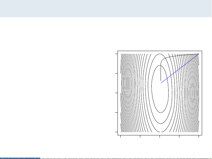
Newton’s method

x2)

−

1 + x 2

2 )/2 + 5 log(1 + e−

Consider minimizing f (x) = (10x 2

We compare gradient de- scent (black) to Newton’s method (blue), where both take steps of roughly same length

Linearized optimality condition

2f (x)v .

From B & V page 486

f (x + v ) = 0. Let F (x) = ∇ Aternative interpretation of Newton step at x: we seek a direction f (x). Consider linearizing v so that ∇ x), i.e., F (x) + DF (x)(y F around x, via approximation F (y ) − 0 = f (x + v ) ≈ f (x) + ∇ Solving for v yields v = ∇ f (x). ≈ ∇ 1 2f (x))− ∇ ( ∇ −

History: work of Newton (1685) and Raphson (1690) originally focused on finding roots of polynomials. Simpson (1740) applied this idea to general nonlinear equations, and minimization by setting the gradient to zero.

Affine invariance of Newton’s method

Rn ∈ Important property Newton’s method: affine invariance. Given f , n. Let x = Ay , and g (y ) = f (Ay ). Newton nonsingular A steps on g are

2g (y ))−

y + = y − = y f (Ay ) − = y ( ∇ (AT ∇ 1( ∇ f (Ay ) A− g (y ) ∇ 1AT 2f (Ay )A)− 1 2f (Ay ))− − ∇ ∇ Hence

1 2f (Ay ))−

Ay + = Ay f (Ay ), ( ∇ − ∇ i.e.,

1f (x).

2f (x))−

x + = x ( −

∇ So progress is independent of problem scaling; recall that this is not true of gradient descent.

Newton decrement

At a point x, we define the Newton decrement as

1 2f (x))−

(cid:16) (cid:17)1/2 . λ(x) = f (x)T ( f (x) ∇ ∇ ∇

2f (x)(y

2f (x))−

This relates to the difference between f (x) and the minimum of its quadratic approximation: (cid:18) (cid:19) f (x) f (x) + f (x)T (y x) + (y x)T x) min y 1 2 − ∇ − − − ∇ (cid:18) (cid:19) = f (x) f (x) f (x)T ( f (x) − 1 2 ∇ − ∇ ∇

= λ(x)2. 1 2

Therefore can think of λ2(x)/2 as an approximate upper bound on the suboptimality gap f (x) f ∗. −

Newton decrement

2f (x))−

Another interpretation of Newton decrement: if Newton direction is v = f (x), then ( ∇ −

2f (x)v )1/2 =

2f (x),

v ∇ λ(x) = (v T (cid:107) (cid:107)∇ ∇

2f (x).

i.e., λ(x) is the length of the Newton step in the norm defined by the Hessian ∇

Note that the Newton decrement, like the Newton steps, are affine invariant; i.e., if we defined g (y ) = f (Ay ) for nonsingular A, then λg (y ) would match λf (x) at x = Ay .

Backtracking line search

So far what we’ve seen is called pure Newton’s method. This need not converge. In practice, we use damped Newton’s method (i.e., Newton’s method), which repeats

2f (x))−

x + = x t( f (x). − ∇ ∇ Note that the pure method uses t = 1.

α ≤ Step sizes here typically are chosen by backtracking search, with 1/2, 0 < β < 1. At each iteration, we start parameters 0 ≤ with t = 1 and while

f (x + tv ) > f (x) + αt f (x)T v , ∇

2f (x))−

we shrink t = βt, else we perform the Newton update. Note that here v = f (x)T v = f (x), so λ2(x). ∇ ∇ − ( − ∇

Example: logistic regression

Logistic regression example, with n = 500, p = 100: we compare gradient descent and Newton’s method, both with backtracking

Newton’s method: in a totally different regime of convergence...!

Convergence analysis

(cid:73)

Assume that f convex, twice differentiable, having dom(f ) = Rn, and additionally

∇

f is Lipschitz with parameter L. (cid:73) f is strongly convex with parameter m. 2f is Lipschitz with parameter M. (cid:73)

∇ Theorem Newton’s method with backtracking line search satisfies the following two-stage convergence bounds

if k   γk k0 − f (x (k)) f ∗ f ∗) − (cid:1)2k−k0+1 − ≤  ≤ if k > k0. (f (x (0)) (cid:0) 1 2m3 M 2 2

2α) m2/M, and k0 is the } − 2 < η. (cid:107)∇ Here γ = αβ2η2m/L2, η = min 1, 3(1 { f (x (k0+1)) number of steps until (cid:107)

Convergence analysis

(cid:73) Damped phase:

m2/M ≤ In more detail, convergence analysis reveals γ > 0, 0 < η such that convergence follows two stages

(cid:73) Pure phase:

2 (cid:107)

η, and (cid:107)∇ f (x (k)) (cid:107) f (x (k+1)) ≥ f (x (k)) γ. − ≤ − < η, backtracking selects t = 1, and f (x (k)) (cid:107) (cid:107)∇ (cid:19)2 (cid:18) M . f (x (k+1)) M 2m2 (cid:107)∇ ≤ 2m2 (cid:107)∇ f (x (k)) (cid:107)

Note that once we enter pure phase, we won’t leave, because

(cid:19)2 (cid:18) M η 2m2 M 2m2 η ≤

when η m2/M. ≤

Convergence analysis

ε, f ∗ ≤ − Unraveling this result, what does it say? To get f (x (k)) we need at most

f ∗ − + log log(ε0/ε, ) f (x (0)) γ

(cid:73) This is called quadratic convergence. Compare this to linear

iterations, where ε0 = 2m3/M 2.

f ∗

convergence (which, recall, is what gradient descent achieves under strong convexity).

−

(cid:73) The above result is a local convergence rate, i.e., we are only guaranteed quadratic convergence after some number of steps k0, where k0

f (x (0)) γ

(cid:73) Somewhat bothersome may be the fact that the above bound depends on L, m, M, and yet the algorithm itself does not ...

. ≤

Self-concordance

(cid:48)(cid:48)(cid:48)

(cid:48)(cid:48)

A scale-free analysis is possible for self-concordant functions: on R, a convex function f is called self-concordant if

f 2f (x) (x)3/2 for all x, | | ≤

and on Rn is called self-concordant if its projection onto every line segment is so.

Theorem (Nesterov and Nemirovskii)

Newton’s method with backtracking line search requires at most

C (α, β)(f (x (0)) f ∗) + log log(1/ε), −

f ∗, where C (α, β) is a constant that − iterations to reach f (x (k)) only depends on α, β.

Self-concordance

What kind of functions are self-concordant?

(cid:73) f (x) =

(cid:73) f (X ) =

i=1 log(xi ) on Rn log(det(X )) on Sn

++. ++.

(cid:80)n −

(cid:73) If g is self-concordant, then so is f (x) = g (Ax + b).

(cid:73) In the definition of self-concordance, we can replace factor of

−

(cid:73) If g is κ-self-concordant, then we can rescale: f (x) = κ

4 g (x) is

2 by a general κ > 0.

self-concordant (2-self-concordant).

Comparison to first-order methods

(cid:73) Memory: each iteration of Newton’s method requires O(n2)

At a high-level:

(cid:73) Computation: each Newton iteration requires O(n3) flops

n Hessian); each gradient iteration requires O(n) × storage (n storage (n-dimensional gradient).

n linear system); each gradient iteration ×

(solving a dense n requires O(n) flops (scaling/adding n-dimensional vectors). (cid:73) Backtracking: backtracking line search has roughly the same

(cid:73) Conditioning: Newton’s method is not affected by a problem’s

cost, both use O(n) flops per inner backtracking step.

conditioning, but gradient descent can seriously degrade. (cid:73) Fragility: Newton’s method may be empirically more sensitive to bugs/numerical errors, gradient descent is more robust.

Newton method vs. gradient descent

Back to logistic regression example: now x-axis is parametrized in terms of time taken per iteration

Each gradient descent step is O(p), but each Newton step is

O(p3).

Sparse, structured problems

When the inner linear systems (in Hessian) can be solved efficiently and reliably, Newton’s method can strive.

2f (x) is sparse and structured for all x, say banded, then E.g., if both memory and computation are O(n) with Newton iterations.

∇

(cid:73) If g (β) = f (X β), then

2g (β) = X T

2f (X β)X . Hence if X

What functions admit a structured Hessian? Two examples:

2g is structured.

∇ is a structured predictor matrix and ∇ 2f is diagonal, then ∇

2f is diagonal,

(cid:73) If we seek to minimize f (β) + g (Dβ), where

∇

2f ∗(

g is not smooth, and D is a structured penalty matrix, then u). Often the Lagrange dual function is D T u) g ∗( f ∗( − − − − D D T u)D T can be structured. − ∇ −

Quasi-Newton methods

2f (x) with H

∇ (cid:31) If the Hessian is too expensive (or singular), then a quasi-Newton 0, and we method can be used to approximate update according to

1 tH −

(cid:73) Approximate Hessian H is recomputed at each step. Goal is to

1 cheap to apply (possibly, cheap storage too).

x + = x f (x). − ∇

(cid:73) Convergence is fast: superlinear, but not the same as Newton. Roughly n steps of quasi-Newton make same progress as one Newton step.

(cid:73) Very wide variety of quasi-Newton methods; common theme is

make H −

to “propogate” computation of H across iterations.

Quasi-Newton methods

1 via rank 2 updates from previous iterations;

(cid:73) Update H, H −

1 is simply O(n2) flops.

Davidon-Fletcher-Powell or DFP:

cost is O(n2) for these updates. (cid:73) Since it is being stored, applying H − (cid:73) Can be motivated by Taylor series expansion.

(cid:73) Came after DFP, but BFGS is now much more widely used. 1 via rank 2 updates, but does so in a (cid:73) Again, updates H, H −

Broyden-Fletcher-Goldfarb-Shanno or BFGS:

(cid:73) Also has a limited-memory version, L-BFGS: instead of letting updates propogate over all iterations, only keeps updates from last m iterations; storage is now O(mn) instead of O(n2).

“dual” fashion to DFP; cost is still O(n2).

References and further reading

S. Boyd and L. Vandenberghe (2004), Convex optimization, Chapters 9 and 10

Y. Nesterov (1998), Introductory lectures on convex optimization: a basic course, Chapter 2

Y. Nesterov and A. Nemirovskii (1994), Interior-point polynomial methods in convex programming, Chapter 2

J. Nocedal and S. Wright (2006), Numerical optimization, Chapters 6 and 7

L. Vandenberghe, Lecture notes for EE 236C, UCLA, Spring 2011-2012

Bài giảng Tối ưu hóa nâng cao: Chương 10 - Hoàng Nam Dũng