HPU2. Nat. Sci. Tech. Vol 03, issue 02 (2024), 59-69.
HPU2 Journal of Sciences: Natural Sciences and Technology
Journal homepage: https://sj.hpu2.edu.vn
Article type: Research article
A convergence enhancement approach for tomographic reconstruction in ultrasonic tomography
Quang-Huy Trana*, Minh-Duc Daoa, Manh-Quang Vua, The-Lam Nguyena, Thi-Theu Luongb
aHanoi Pedagogical University 2, Vinh Phuc, Vietnam bHoa Binh University, Hanoi, Vietnam
Abstract
Ultrasound tomography is a non-invasive imaging technique that seeks to determine the internal distribution of acoustic properties within the body by analyzing measured ultrasound data. Based on the distorted Born iterative method (DBIM), this work suggests employing resolution-jumping and beamforming techniques for tomographic ultrasound imaging. The beamforming technique leverages multiple transmitting elements from the ultrasound probe, operating concurrently, to generate a focused and narrow beam. This targeted approach helps in reducing noise, thus enhancing the quality of the collected data. Meanwhile, resolution-jumping optimizes the imaging process by adjusting the resolution dynamically, thereby improving both the quality and speed of the reconstruction. The benefits of the proposed method are evident in the results of numerical simulations, which demonstrate a substantial improvement in the quality of image recovery. These simulations also highlight a significant reduction in the total runtime required for imaging, showcasing the efficiency of the approach. By combining these advanced methods, the work offers a promising pathway toward more accurate and faster tomographic ultrasound imaging, which could lead to better diagnostic capabilities in medical applications.
Keywords: Inverse scattering, beamforming, interpolation, ultrasound tomography, distorted Born iterative method
1. Introduction
An imaging method called ultrasound tomography uses acoustic fields to provide images in heterogeneous media. It involves the reconstruction of cross-sections of the internal structures of the
* Corresponding author, E-mail: tranquanghuy@hpu2.edu.vn
https://doi.org/10.56764/hpu2.jos.2024.3.2.59-69
Received date: 27-4-2024 ; Revised date: 02-7-2024 ; Accepted date: 06-7-2024
This is licensed under the CC BY-NC 4.0
59
HPU2. Nat. Sci. Tech. 2024, 3(2), 59-69
body by linearizing the non-linear wave equation and applying the Born or Rytov approximation. It is particularly useful for imaging soft tissues and is commonly employed in various medical applications, including breast imaging, liver imaging, and vascular imaging. Diffraction tomography is a specific type of ultrasound tomography that utilizes the generalized Fourier slice theorem for image reconstruction 0. Ultrasonic computed tomography (UCT) is another approach that numerically solves the inverse scattering issue associated with the forward scattering issue in inhomogeneous media. Various approximations can be used depending on the level of inhomogeneity, such as the straight ray approximation or high-order approximations [2]. Acoustic travel-time tomography is a remote sensing technique that measures temperature and flow fields by analyzing the dependence of sound speed on temperature and wind speed. It can be used to reconstruct three-dimensional distributions of temperature and flow fields without the need for sensors 0.
Research on ultrasound tomography utilizes various methodologies. One common approach is the distorted Born iterative method (DBIM), which uses inverse scattering techniques to detect small targets by analyzing sound contrast or attenuation 0–0. Another methodology is the use of the truncated total least squares (TTLS) and regularized total least squares (RTLS-Newton) algorithms to solve the ill-posed linear system of inverse scatter equations 0. Additionally, signal processing methods such as wavelet-based or energy-based methods are employed to determine the time of flight (TOF) in ultrasound tomography 0. The acoustic wave equation in the time domain is tackled using the finite element method, followed by the comparison of numerical results with experimental data 0. Additionally, a wavelet transform-based adaptive filtering algorithm is introduced to enhance filtering and denoising efficacy in tomography systems 0.
60
https://sj.hpu2.edu.vn
Beamforming is a technique widely used in ultrasound imaging, including ultrasound tomography. It involves combining signals from multiple transducers to enhance the quality and resolution of the resulting image 0. Beamforming in ultrasound tomography offers numerous advantages, including improved resolution, enhanced image quality, increased penetration depth, customizable imaging parameters, real-time imaging capabilities, and optimal SNR. These features collectively contribute to the effectiveness and versatility of ultrasound tomography in medical imaging applications. Nearest neighbor interpolation is a simple and computationally efficient method used in image processing, including ultrasound tomography. While it may not be the most sophisticated interpolation technique, it does have some advantages in specific contexts. Nevertheless, it's essential to emphasize that the choice of interpolation method depends on the specific requirements and characteristics of the imaging application. Nearest neighbor interpolation is computationally less intensive compared to more complex interpolation methods 0. In real-time or near-real-time imaging applications, where speed is critical, the simplicity of nearest neighbor interpolation can be advantageous. Therefore, this study proposes the use of resolution-jumping and beamforming techniques for tomographic image reconstruction. The beamforming approach utilizes multiple probe transmitting elements concurrently to create a focused beam, thereby minimizing noise. Concurrently, resolution-jumping is used to boost the quality and speed of the reconstruction process. The outcomes from numerical simulations indicate a significant enhancement in image recovery quality, as well as a marked decrease in overall imaging time.
HPU2. Nat. Sci. Tech. 2024, 3(2), 59-69
2. Methodology
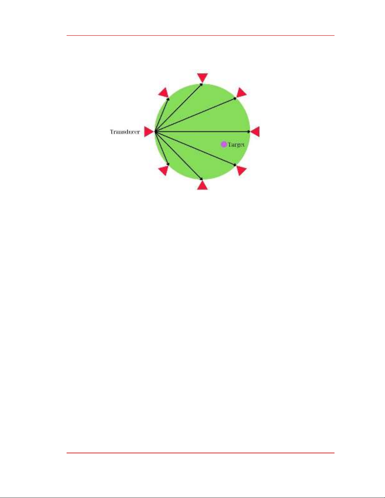
Figure 1. The ultrasonography imaging system's transducer arrangement.
2.1. Distorted Born iterative method
For collecting scattered data, we establish a transducer setup, as shown in Figure 1, assuming the presence of Nr receivers and Nt transmitters. These transmitters Nt are strategically positioned at various angles around the object to capture comprehensive information about it. The ultrasonic signal reception and transmission follow this procedure: Initially, the first three transmitters' ultrasonic waves are simultaneously captured by all receivers (Nr), while the remaining transmitters remain inactive. This assembly of measurements (i.e., 1×Nr measurements) is employed to determine the original transmitter positions. Subsequently, the process is repeated with the next set of three transmitters, with all receivers detecting scattering signals at the second set of transmitter locations. This results in a subsequent set of measurements, totaling 2×Nr measurements. The identical procedure is then applied to the remaining transmitters. Once the measurement process is completed, we acquire Nt/3 sets of collected values, totaling Nt×Nr/3 measurements. In order to achieve a holistic perspective of the object from multiple angles, the results obtained from these Nt/3 sets are integrated.
The integral equation can be used to describe the propagation of waves in an inhomogeneous medium 0, 0:
(1) dr⃗(cid:4593)θ(r⃗(cid:4593))p(r⃗(cid:4593))G(cid:2868)(r⃗, r⃗(cid:4593)) σ(r⃗) = σ(cid:2919)(cid:2924)(cid:2913)(r⃗) + (cid:3505) (cid:2960)
61
https://sj.hpu2.edu.vn
where 𝛔(𝐫⃗) denotes the acoustic pressure, while 𝛔𝐢𝐧𝐜(𝐫⃗) represents the incident field. 𝐆𝟎(𝐫⃗, 𝐫⃗(cid:4593)) is the Green's function associated with a background environment characterized by wave number 𝐤𝟎. The function 𝛉(𝐫⃗) contains details about the acoustic properties of the imaging target. When 𝟐(cid:3439). Using the method of considering constant density and negligible attenuation, 𝛉 = (cid:3435)𝐤𝟐(𝐫⃗) − 𝐤𝟎 moments (MoM), Equation (1) can undergo discretization, enabling its representation in matrix form for both the pressure field within the computational domain, denoted as 𝛔‾ , and the scattered field outside the computational domain, represented as 𝛔‾ sc, as follows:
HPU2. Nat. Sci. Tech. 2024, 3(2), 59-69
σ‾ = (I‾ − C‾ ⋅ 𝒟(θ(cid:3364)))(cid:2879)(cid:2869) ⋅ σ(cid:3365)(cid:2919)(cid:2924)(cid:2913) (2)
σ‾ sc = B‾ ⋅ 𝒟(θ(cid:3364)) ⋅ σ‾ (3)
here 𝐁‾ is a matrix containing Green's coefficients that describe the influence of each pixel on the receivers, while 𝐂‾ is a matrix encompassing Green's coefficients across all pixels. Additionally, 𝓓 is an operator that converts a vector into a diagonalized matrix. Discretizing Equation (1) applied to both 2-D and 3-D scenarios was carried out using sinc basis and delta testing functions 0.
(cid:2870)
An iterative algorithm is utilized to reconstruct the object function from the scattered field data. The process begins with an initial trial function 𝛉(cid:3365)(𝟎), and the corresponding scattered field is calculated based on this initial guess. The object function is then refined iteratively according to the update equation as 𝛉(cid:3365)(𝐧(cid:2878)𝟏) = 𝛉(cid:3365)(𝐧) + 𝚫𝛉(cid:3365)(𝐧), where 𝚫𝛉(cid:3365)(𝐧) is the change in the object function for the nth iteration. This change is determined by solving a regularized optimization problem, which aims to minimize the difference between the measured and calculated scattered fields while incorporating regularization terms to ensure stability and convergence:
(cid:2870)
(cid:2940)𝒪(cid:3364)
Δθ((cid:2924)) = argmin + γ ∥ Δθ(cid:3364) ∥(cid:2870) (cid:2870) ∥∥Δσ‾ sc − H‾ ((cid:2924)) ⋅ Δθ(cid:3364)∥∥ (4)
(cid:2879)(cid:2869)
where the term 𝚫𝛔‾ sc represents the discrepancy among the predicted and measured scattered fields, while the regularization parameter 𝛄 controls the trade-off between data fidelity and model stability. The Frechet derivative matrix 𝐇‾ (𝐧) is structured as follows 0:
⋅ 𝒟(σ‾ ) H‾ ((cid:2924)) = B‾ ⋅ (cid:3419)I‾ − 𝒟(cid:3435)θ(cid:3364)((cid:2924))(cid:3439) ⋅ C‾ (cid:3423) (5)
(cid:2870)max(cid:3419)10(cid:2922)(cid:2925)(cid:2917)(cid:3118) (cid:2902)(cid:2902)(cid:2889), 10(cid:2879)(cid:2872)(cid:3423)
The iterative process continues until the relative residual error (RRE) meets the desired termination tolerance. The RRE is calculated as RRE = ∥∥𝚫𝛔‾ sc ∥∥𝟐/∥∥𝛔‾ sc ∥∥𝟐, where ∥∥𝚫𝛔‾ sc ∥∥𝟐 denotes the 2-norm of the variance between the predicted and measured scattered fields. The regularization parameter 𝛄 is determined based on the method outlined in 0:
γ = 0.5σ(cid:2868) (6)
𝟐, is computed using the power iteration method in conjunction with Rayleigh quotient estimation. This approach provides an efficient way to estimate the largest singular value and its corresponding square. The quality of the reconstructions is assessed by calculating the mean average error (MAE). The MAE is calculated based on the difference between the reconstructed speed of sound contrasts 𝚫𝐜ˆ and the ideal speed of sound contrasts 𝚫𝐜. This metric quantifies the average deviation between the reconstructed and ideal values, providing a measure of the accuracy and effectiveness of the reconstruction process as follows:
where the square of the dominant singular value of 𝐇‾ (𝐧), denoted as 𝛔𝟎
(7) MAE = ∥ Δcˆ − Δc ∥(cid:2869) ∥ Δc ∥(cid:2869)
62
https://sj.hpu2.edu.vn
The single-frequency DBIM may experience divergence issues when the excess phase magnitude Δϕ accumulates from the acoustic wave as it travels through the scatterer approaches π 0. In the case of a homogeneous sphere, Δϕ shown in Eq. (8) can be estimated based on factors such as
HPU2. Nat. Sci. Tech. 2024, 3(2), 59-69
the size of the sphere, the speed of sound in the sphere relative to the surrounding medium, and the frequency of the acoustic wave. This estimation helps determine whether the phase shift is within a tolerable range for the method to remain stable and accurate.
(cid:2879)(cid:2869) − 1)
(8) Δϕ = 2k(cid:2868)a(c(cid:2928)
where the relative speed of sound, denoted as 𝐜𝐫 = 𝐜/𝐜𝟎, measures the speed of sound in the scatterer 𝐜 relative to the speed of sound in the surrounding medium 𝐜𝟎. For a homogeneous sphere with radius 𝐚, the excess phase |𝚫𝛟| accumulated from the acoustic wave while passing through the sphere can be estimated using these parameters. When applying the linearized first-order Born approximation, the quality of the reconstructions can degrade even when the absolute value of 𝚫𝛟 is smaller than 𝛑 0. As a result, any scattering object for which |𝚫𝛟| > 𝛑 is considered to possess a significant acoustic contrast and may pose challenges for accurate reconstruction due to the higher likelihood of divergence.
Nearest neighbor interpolation is the simplest and most commonly used interpolation method. It is computationally less intensive compared to more sophisticated interpolation methods like bilinear or cubic interpolation. The algorithm is easy to implement and requires minimal computational resources. The new pixel takes the value of the original pixel closest to it and does not consider other values in all neighboring points. The distance between two points is often measured as the Euclidean distance or Minkowski distance with k = 2. Kernel function of the nearest neighbor interpolation method 0 is shown as:
1 |x| ≤ 1 2 h(x) = (cid:3422) (9) 0 ≤ |x| 1 2
Figure 2. Illustration of calculating new pixels (u,v) using the nearest neighbor interpolation method.
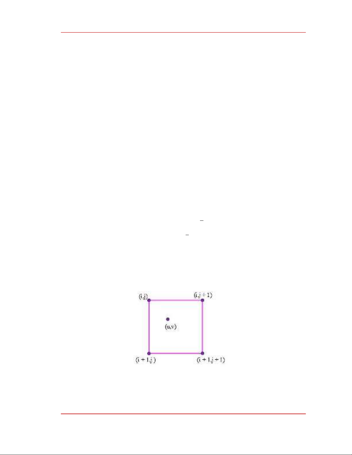
where, x is the distance between the interpolation point and the grid point. Suppose that we have a pixel (u,v) with four neighbours (i, j), (i, j + 1), (i + 1, j) and (i + 1, j + 1), and values f(i, j), f(i, j + 1), f(i + 1, j), f(i + 1, j + 1) as shown in Figure 2. The distance between (u,v) and (i, j), (i, j + 1), (i + 1, j), (i + 1, j + 1) will be calculated, the value at (u, v) will be assigned the value of the point closest to it.
63
https://sj.hpu2.edu.vn
The image restoration procedure comprises two distinct phases: In the initial stage, the object is reconstructed with low resolution (N1×N1) during the initial iterations employing the beamformed approach. This initial stage employs lower resolution to facilitate rapid convergence. Subsequently, in
HPU2. Nat. Sci. Tech. 2024, 3(2), 59-69
the second stage, the object is reconstructed with high resolution (N2×N2) during the remaining iterations, still utilizing the beamformed approach. Using high resolution is implemented to get the desired image resolution. Expanding the dimensions of an image can be achieved through a technique known as nearest-neighbor interpolation, where each pixel is replaced by four pixels of equal intensity. This process enlarges the image without sacrificing its inherent details. Notably, nearest-neighbor interpolation boasts a straightforward implementation and consumes minimal processing time. While various interpolation techniques exist, such as bilinear, bicubic, and spline interpolation, among others, we select nearest-neighbor interpolation mainly because of its time efficiency and its avoidance of the need to generate new data. Normalized error and noise reduction are shown by the obtained results of the proposed approach.
2.2. Numerical simulation and discussion
a)
b)
a)
b)
10
10
)
)
%
%
8
8
6
6
4
4
( t s a r t s n o c
( t s a r t s n o c
2
2
d n u o S
d n u o S
0
0
2
2
2
2
0
0
0
0
-2
-2
-2
-2
Number of pixels
Number of pixels
Figure 3. Ideal target function for a) N=9 and b) N=18.
Figure 4. presents the normalized error differentiation between the beamforming-DBIM and beamforming- interpolation-DBIM after each iteration in the case of Nt = 15, Nr = 15, N = 18, or Nt×Nr = 0.694N2. Initially, the beamforming-DBIM approach starts with a higher normalized error compared to the beamforming-interpolation- DBIM approach. As iterations progress, both approaches show a decrease in their normalized error values, indicating improvement in performance. The beamforming-interpolation-DBIM approach consistently maintains a lower normalized error compared to the beamforming-DBIM approach throughout all iterations. Towards the end of the iterations, the difference in normalized error between the two approaches becomes smaller, but the the beamforming-DBIM approach. beamforming-interpolation-DBIM approach consistently outperforms Overall, the trend suggests that the beamforming-interpolation-DBIM approach tends to converge to a lower normalized error faster and maintains a better performance throughout the iterations compared to the beamforming-DBIM approach.
Notably, in the third iteration of the beamforming-interpolation-DBIM method, the normalization error reaches its minimum. This is understandable because in the first 3 iterations, the image restoration process is performed with low resolution (N1×N1). That is, the number of variables is small, while the number of measurements remains constant, so the normalization error is minimized at this stage. However, what we want is to restore the image with high resolution (N2×N2) starting from the fourth iteration. This shows that estimating the target in the first iterations is very essential to achieve convergence speed and the beamforming-
64
https://sj.hpu2.edu.vn
Simulation parameters: Transmitter frequency sets at 1 MHz, sound contrast of 10%, object diameter 7.3 mm, transducer-to-object distances spanning 100 mm, background environment's sound velocity established at 1540 m/s, the number of pixels along an axis is N, a total of 8 iterations (with iterations for N1×N1 denoted as NN1 = 3 and for N2×N2 denoted as NN2 = 5), and a 10% level of noise. Figure 3. indicates the ideal target function that needs to be recovered.
HPU2. Nat. Sci. Tech. 2024, 3(2), 59-69
interpolation-DBIM method has proven quite effective. Moreover, the total runtimes of the beamforming-DBIM and the beamforming-interpolation-DBIM are 13.608345 and 9.062086 seconds, respectively. Hence, the reduced percentage of the total runtime for beamforming-interpolation-DBIM compared to the beamforming- DBIM is approximately 33.41%. This indicates that the beamforming-interpolation-DBIM outperforms the beamforming-DBIM in terms of total runtime, completing its execution faster.
0.8
Beamforming-DBIM Beamforming-Interpolation-DBIM
0.7
0.6
0.5
r o r r e d e z
0.4
i l
0.3
a m r o N
0.2
0.1
0
1
2
3
4
5
6
7
8
Number of iterations
Figure 4. The normalized error differentiation between the beamforming-DBIM and beamforming-interpolation- DBIM after each iteration in case of Nt = 15, Nr = 15, N = 18, or Nt×Nr = 0.694N2.
1
0.9
Beamforming-DBIM Beamforming-Interpolation-DBIM
0.8
0.7
0.6
r o r r e
0.5
d e z
i l
0.4
a m
r o N
0.3
0.2
0.1
0
1
2
3
4
5
6
7
8
Number of iterations
Figure 5. The normalized error differentiation between the beamforming-DBIM and beamforming-interpolation- DBIM after each iteration in the case of Nt = 20, Nr = 20, N = 18, or Nt×Nr = 1.235N2.
65
https://sj.hpu2.edu.vn
HPU2. Nat. Sci. Tech. 2024, 3(2), 59-69
a)
b)
b)
a)
10
10
)
)
%
%
8
8
6
6
4
4
( t s a r t s n o c
( t s a r t s n o c
2
2
d n u o S
d n u o S
2
2
2
2
0
0
0
0
-2
-2
-2
-2
c)
d)
c)
d)
)
10
10
)
%
%
8
8
6
6
4
( t s a r t s n o c
4
( t s a r t s n o c
2
2
d n u o S
d n u o S
2
2
2
2
0
0
0
0
-2
-2
-2
-2
Number of pixels
Number of pixels
e)
f)
e)
f)
12
)
10
)
%
%
10
8
8
6
6
4
( t s a r t s n o c
( t s a r t s n o c
4
2
2
d n u o S
d n u o S
2
2
2
2
0
0
0
0
-2
-2
-2
-2
Number of pixels
Number of pixels
g)
h)
g)
h)
12
)
10
)
%
%
10
8
8
6
6
4
( t s a r t s n o c
( t s a r t s n o c
4
2
2
d n u o S
d n u o S
2
2
2
2
0
0
0
0
-2
-2
-2
-2
Number of pixels
Figure 6. Reconstructed target function of the beamforming-DBIM (a, c, e, and g) and beamforming- interpolation-DBIM (b, d, f, and h) after first (a and b), third (c and d), fifth (e and f), and eighth (g and h) iterations when Nt= Nr= 15.
66
https://sj.hpu2.edu.vn
HPU2. Nat. Sci. Tech. 2024, 3(2), 59-69
a)
b)
b)
a)
)
8
)
8
%
%
6
6
4
4
( t s a r t s n o c
( t s a r t s n o c
2
2
d n u o S
d n u o S
2
2
2
2
0
0
0
0
-2
-2
-2
-2
Number of pixels
Number of pixels
c)
d)
10
)
)
10
%
%
8
8
6
6
4
4
( t s a r t s n o c
( t s a r t s n o c
2
2
d n u o S
d n u o S
2
2
2
2
0
0
0
0
-2
-2
-2
-2
Number of pixels
Number of pixels
e)
f)
e)
f)
12
)
)
10
%
%
10
8
8
6
6
4
( t s a r t s n o c
( t s a r t s n o c
4
2
2
d n u o S
d n u o S
2
2
2
2
0
0
0
0
-2
-2
-2
-2
g)
h)
g)
c) d)
)
12
10
)
%
%
10
8
8
6
6
( t s a r t s n o c
4
( t s a r t s n o c
4
2
2
d n u o S
d n u o S
2
2
2
2
0
0
0
0
-2
-2
-2
-2
Number of pixels
Number of pixels
Figure 7. Reconstructed target function of the beamforming-DBIM (a, c, e, and g) and beamforming- interpolation-DBIM (b, d, f, and h) after first (a and b), third (c and d), fifth (e and f), and eighth (g and h) iterations when Nt= Nr= 20.
67
https://sj.hpu2.edu.vn
h)
HPU2. Nat. Sci. Tech. 2024, 3(2), 59-69
The normalized error differentiation between the beamforming-DBIM and beamforming- interpolation-DBIM after each iteration in the case of Nt = 20, Nr = 20, N = 18, or Nt×Nr = 1.235N2 is shown in Figure 5. For the initial error of the first iteration, the beamforming-interpolation-DBIM has a significantly lower initial error compared to the beamforming-DBIM. The error reduction is substantial from the first iteration itself. For the convergence rate, both approaches show a decrease in error with each iteration, indicating convergence towards a solution. However, the beamforming- interpolation-DBIM tends to converge faster, reaching lower error values in fewer iterations compared to the beamforming-DBIM. For stability, the beamforming-interpolation-DBIM appears to have a more stable convergence pattern, with consistent decreases in error across iterations. The beamforming-DBIM, while showing a reduction in error, demonstrates slightly more fluctuations in error values between iterations. For the final error of the last iteration, beamforming-interpolation- DBIM achieves a lower error compared to the beamforming-DBIM, indicating superior performance in terms of accuracy. In general, the beamforming-interpolation-DBIM exhibits a notable improvement over the beamforming-DBIM in terms of both initial error reduction and convergence speed. It consistently maintains a lower error throughout iterations, indicating its effectiveness in producing accurate results more efficiently. The total runtime of the beamforming-DBIM and the beamforming-interpolation-DBIM are 23.192424 and 16.575251 seconds, respectively. Therefore, the reduced percentage of the total runtime for the beamforming-interpolation-DBIM compared to the beamforming-DBIM is approximately 28.53%. This indicates that the beamforming-interpolation- DBIM completes its execution approximately 28.53% faster than the beamforming-DBIM. Figure 6 and Figure 7 show the reconstructed target function of the beamforming-DBIM and beamforming- interpolation-DBIM after the first, third, fifth, and eighth iterations in the case of Nt= Nr= 15 and 20, respectively. Visually, we see that the beamforming-interpolation-DBIM method converges quite well as the number of iterations increases. This is shown by the recovered object function.
3. Conclusions
Ultrasound tomography plays a pivotal role in medical diagnostics, providing non-invasive imaging capabilities for soft tissues with high resolution. This work introduces a novel approach to enhance image reconstruction within the context of diffraction tomography. By integrating techniques of beamforming and interpolation, we aim to improve the convergence rate and image reconstruction quality. By steering the transmitted and received signals toward specific directions, beamforming enhances the signal-to-noise ratio and improves the quality of acquired ultrasound data. Additionally, nearest neighbor interpolation is leveraged for its computational efficiency and simplicity, ensuring rapid processing suitable for real-time applications. Results demonstrate the potential for more accurate information retrieval and improved convergence rate of the imaging target.
[1] F. Schubert, “Basic principles of acoustic emission tomography,” J. Acoustic Emission, vol. 22, pp. 147–158,
2004. [Online]. Available: https://www.ndt.net/article/jae/papers/22-147.pdf.
[2] C. Pintavirooj, K. Jaruwongrungsee, W. Withayachumnankul, K. Hamamoto, and S. Daochai, “Ultrasonic
diffraction tomography: the experimental result,” in WSCG’2005, 2005, pp. 49–50.
[3] Philippe Lasaygues, Régine Guillermin, and J.-P. Lefebvre, “Ultrasonic computed tomography,” in Springer
eBooks, pp. 441–459, Nov. 2010, doi: 10.1007/978-94-007-0017-817.
[4] T. Q. Huy, H. H. Tue, T. T. Long, and T. Duc-Tan, “Deterministic compressive sampling for high-quality image reconstruction of ultrasound tomography,” BMC Med. Imaging, vol. 17, no. 1, May. 2017, doi: 10.1186/s12880-017-0206-8.
68
https://sj.hpu2.edu.vn
References
HPU2. Nat. Sci. Tech. 2024, 3(2), 59-69
[5] Z. Miao and P. Kosmas, “Multiple-frequency DBIM-TwIST algorithm for microwave breast imaging,” IEEE Trans. Antennas Propag., vol. 65, no. 5, pp. 2507–2516, May. 2017, doi: 10.1109/tap.2017.2679067. [6] R. Lavarello and M. L. Oelze, “Density imaging using a multiple-frequency DBIM approach,” IEEE IEEE Trans. Ultrason. Ferroelectr. Freq. Control, vol. 57, no. 11, pp. 2471–2479, Nov. 2010, doi: 10.1109/tuffc.2010.1713.
[7] T. Quang-Huy, K. T. Nguyen, P. T. Doan, and D.-T. Tran, “Interpolated hybrid DBIM approach for enhanced imaging in ultrasound tomography,” Res. Biomed. Eng., vol. 38, no. 2, pp. 389–400, Jan. 2022, doi: 10.1007/s42600-021-00192-x.
[8] L. Guo, M. K. Farsani, A. Stancombe, K. Bialkowski, and A. Abbosh, “Adaptive clustering distorted Born iterative method for microwave brain tomography with stroke detection and classification,” IEEE Trans. Biomed. Eng., vol. 69, no. 4, pp. 1512–1523, Apr. 2021, doi: 10.1109/tbme.2021.3122113.
[9] A. Carevic et al., “Solving the ultrasound inverse scattering problem of inhomogeneous media using different approaches of total least squares algorithms,” in Proc. SPIE 10580, Medical Imaging 2018: Ultrasonic Imaging and Tomography, Mar. 2018, p. 105800J, doi: 10.1117/12.2293627.
[10] L. Zhang et al., “The identification of accurate and computationally efficient arrival time pick-up method for acoustic tomography,” in Nondestructive characterization and monitoring of advanced materials, aerospace, civil infrastructure, and transportation XIII, Proceedings of the SPIE, Vol. 10971, Apr. 2019, p. 1097114, doi: 10.1117/12.2515403.
[11] R. M. Nakanishi, “Comparison of experimental and numerical simulation data of ultrasound signals,” M. S. thesis, Dept. of Polytechnic School, University of Sao Paulo, Sao Paulo, Brazil, 2019, doi:10.11606/D.3.2020.tde-08012020-162233.
[12] R. Wang, Y. Gao, M. Zhang, Y. Sun, and H. Li, “Research on tomography system for ultrasonic process of particle two-phase flow based on adaptive filtering.,” in ICISCAE (IEEE), 2021, pp. 404–409, doi: 10.1109/iciscae52414.2021.9590729.
[13] T. Szasz, A. Basarab, and D. Kouame, “Beamforming through regularized inverse problems in ultrasound medical imaging,” IEEE Trans. Ultrason. Ferroelectr. Freq. Control, vol. 63, no. 12, pp. 2031–2044, Dec. 2016, doi: 10.1109/tuffc.2016.2608939.
[14] D. Han, “Comparison of commonly used image interpolation methods,” in Proceedings of the 2nd International Conference on Computer Science and Electronics Engineering (ICCSEE 2013), Jan. 2013, doi: 10.2991/iccsee.2013.391.
[15] W. C. Chew and Y. M. Wang, “Reconstruction of two-dimensional permittivity distribution using the distorted Born iterative method,” IEEE Trans. Med. Imaging, vol. 9, no. 2, pp. 218–225, Jun. 1990, doi: 10.1109/42.56334.
[16] D. Borup, “Nonperturbative diffraction tomography via Gauss-Newton iteration applied to the scattering integral equation,” Ultrason. Imaging, vol. 14, no. 1, pp. 69–85, Jan. 1992, doi: 10.1016/0161- 7346(92)90073-5.
[17] M. L. Tracy and S. A. Johnson, “Inverse scattering solutions by a sine basis, multiple source, moment method—Part II: Numerical evaluations,” Ultrason. Imaging, vol. 5, no. 4, pp. 376–392, 1983, doi: 10.1177/016173468300500407.
[18] R. J. Lavarello and M. L. Oelze, “Density imaging using inverse scattering,” J. Acoust. Soc. Am., vol. 125,
no. 2, pp. 793–802, Feb. 2009, doi: 10.1121/1.3050249.
[19] T. J. Cavicchi, S. A. Johnson, and W. D. O’Brien, “Application of the sinc basis moment method to the reconstruction of infinite circular cylinders,” IEEE Trans. Ultrason. Ferroelectr. Freq. Control, vol. 35, no. 1, pp. 22–33, Jan. 1988, doi: 10.1109/58.4144.
[20] M. Slaney, A. C. Kak, and L. E. Larsen, “Limitations of Imaging with First-Order Diffraction Tomography,” IEEE Trans. Microw. Theory Tech., vol. 32, no. 8, pp. 860–874, Aug. 1984, doi: 10.1109/tmtt.1984.1132783.
69
https://sj.hpu2.edu.vn