Forecasting exports and imports through artificial neural network and autoregressive integrated moving average

Chia sẻ: Huỳnh Lê Khánh Thi | Ngày: | Loại File: PDF | Số trang:12

Thêm vào BST

Báo xấu

6
lượt xem 0
download

Download Vui lòng tải xuống để xem tài liệu đầy đủ

In this study, total annual exports and imports of the Kingdom of Saudi Arabia are forecasted using Artificial Neural Network (ANN) and Autoregressive Integrated Moving Average (ARIMA) models.

Chủ đề:

Bình luận(0) Đăng nhập để gửi bình luận!

Lưu

Nội dung Text: Forecasting exports and imports through artificial neural network and autoregressive integrated moving average

Decision Science Letters 8 (2019) 249–260 Contents lists available at GrowingScience Decision Science Letters homepage: www.GrowingScience.com/dsl Forecasting exports and imports through artificial neural network and autoregressive integrated moving average Teg Alama* aCollege of Business Administration, Prince Sattam bin Abdulaziz University, Al Kharj, Kingdom of Saudi Arabia CHRONICLE ABSTRACT Article history: Nowadays, Saudi government has established several strategic tactics such as Saudi Vision 2030 Received January 2, 2019 to predict the future of the country. In order to accomplish a superior growth in the economy of Received in revised format: the country, mathematical model and forecasting techniques are important tools. In this study, January 28, 2019 total annual exports and imports of the Kingdom of Saudi Arabia are forecasted using Artificial Accepted February 14, 2019 Available online Neural Network (ANN) and Autoregressive Integrated Moving Average (ARIMA) models. This February 14, 2019 paper tries to predict a time series data using ANN and ARIMA models on total annual exports Keywords: and imports of Kingdom of Saudi Arabia from the year 1968 to the year 2017 with the help of Artificial Neural Networks (ANN) statistical software XLSTAT. The applied models are used to predict some future values of total Autoregressive Integrated Moving annual exports and imports of the Kingdom of Saudi Arabia. It is found that the ANN and Average (ARIMA) ARIMA (1, 1, 2) and ARIMA (0, 1, 1) models are suitable for predicting the total annual exports Forecasting and imports of the Kingdom of Saudi Arabia. Export and Import Kingdom of Saudi Arabia © 2018 by the authors; licensee Growing Science, Canada. 1. Introduction The Kingdom of Saudi Arabia preserves the largest amount of export of petroleum and it has the second-largest proven petroleum and the fifth-largest proven natural gas reserves in the world. The economy of the country depends primarily on oil and gas products. Saudi Arabia exported SAR 611.48B and imported SAR491.43B in 2016, yielding a positive trade balance of SAR 119.29B. The growth domestic product (GDP) of Saudi Arabia was SAR 2423.40B and its GDP per capita was SAR 204.08K. 2. Methods and Materials 2.1 Artificial Neural Network Artificial Neural Network (ANN) is a well-organized data mining technique which is achieved from a biological neural networks. ANN collects a large amount of data interconnected in some specific patterns to help communication among various units normally called nodes or neurons and each of these is joint with other neurons through some connection links. Each association is joint with a particular weight, which gives some feedback about the input data. This is an essential part of neurons * Corresponding author. E-mail address: t.alam@psau.edu.sa (T. Alam) © 2019 by the authors; licensee Growing Science, Canada. doi: 10.5267/j.dsl.2019.2.001
250 to come up with a particular problem. Each neuron maintains a combined state or an activation signal. Output signals, produced after joining the input signals and activation rule, are dispatched to other units. Some important developments of ANN are given in Table 1. Table 1 Some Important Development s of ANN Year Author Development 1943 Warren McCulloch and Walter Physiologist, and mathematician’s ideas are used for ANN purposes Pitts 1956 Taylor An associative memory network 1964 Taylor Winner-take-all circuit with association with output units 1969 Minsky and Papert Multilayer perceptron concept 1971 Kohonen Associative memories 1986 Rumelhart, Hinton, and Williams Generalised Delta Rule 1988 Kosko A hybrid of Binary Associative Memory and Fuzzy Logic ANN 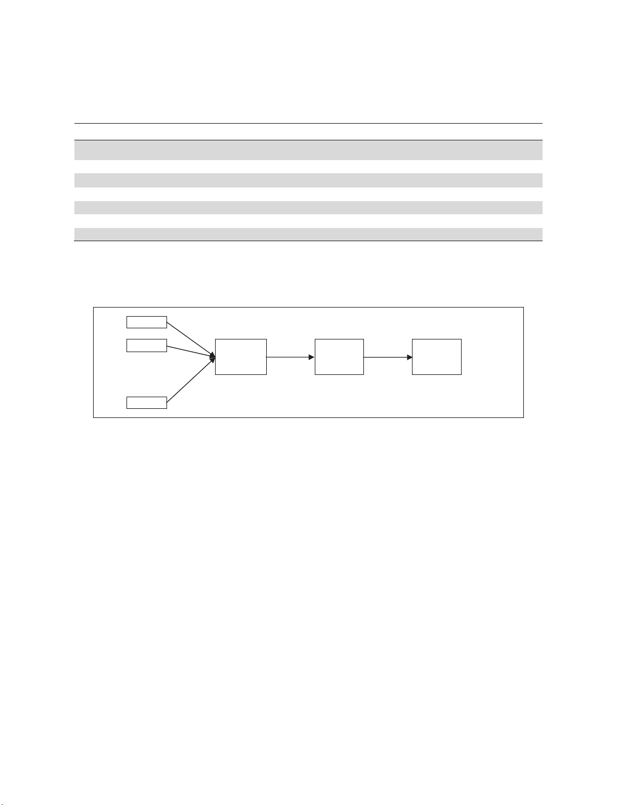2.1.1. Basic Model of Artificial Neural Network An ANN mode can be expressed in Fig. 1 as follows, x1 W1 x2 yin Inputs . W2 Σ ϝ Y Output . . Activation function xm Wm Fig. 1. Neural Network m Any ANN configuration can be computed as yin   wi xi . The output is measured using the function (Y) i 1 based on the net input (F(yin)). ANN has been wiedly used for predicting different incidennts (Gaida et al., 2017; Kotur & Žarković, 2016; Sözen et al., 2011; Deng, 2010; Tektaş, 2010). Kavaklioglu et al. (2009) applied ANN method to estimazte the electricity consumption using the historical data over the period 1976-2006. Ardakani and Ardehali (2014a,b) used ANN for prediction of electrical energy consumption for some countires. Li et al. (2007) applied ANN for estimating crop yield and compared their results with multivariate regression (Chamberlain, 1982). Zeng et al. (2017) implemented enhanced back-propagation for energy consumption predicting using neural network. Sokolov- Mladenović et al. (2016) estimated economic growth using ANN with a learning system based on trade, import and export parameters. Kankal and Uzlu (2017) applied ANN with a metaheuristics method to forecast demand for electricity. Tsai and Huang (2017) applied ANN for forecasting container flows among some Asian ports. According to Aydin et al. (2016), some of the world’s largest energy consumer (HC) consume approximately 62% of the world energy consumption. Thus, it is essential to find a predicted the future of world energy consumption. They proposed an ANN based model for HCs’ energy consumptions. Olgun et al. (2012) applied ANN for predicting the demand of natural gas in Turkey and comparted their results with support vector machines (Joachims, 1998; Uddin, 2009; Hsu & Lin, 2002; Chang & Lin, 2011). Liu et al. (2017) applied ANN to forecast the Chinese energy consumption. Mollaiy-Berneti (2015) used a hybrid of ANN based on the back- propagation (BP) type neural network and some methaheuristics. The method offered some advantage over the local search capabilities of BP technique and some search capability of some metaheuristics algorithm. Panda et al. (2010) used ANN method for the prediction of the agricultural crop yield
T. Alam / Decision Science Letters 8 (2019) 251 prediction. This paper uses ANN technique to estimate the import and export of the Kingdom of Saudi Arabia. 2.1.2. Auto-Regressive Integrated Moving Average (ARIMA) The early time series are concentrated on stochastic processes by Walker (1931). Udny Yule (1927) and Wold (1938) are among the first who introduced Autoregressive Moving Average (ARMA) models for time series, but was not able to determine the likelihood function for maximum likelihood (ML) estimation of the parameters (Ljung & Box, 1978). Then Box and Jenkins (Box et al., 2015) developed their methods for time series for forecasting purposes. Today, most important tools based on Box- Jenkins models (Kendall, 1995; Olajide et al., 2012) are commonly used for forecasting. ARIMA models are the most comprehensive times series for forecasting purposes. The linear type ARIMA model is considered as a primary forecasting one for a stationary data where the predictors includes of lags of the dependent variable and/or lags of the forecast errors. A typical ARIMA model is stated as an ‘ARIMA (p, d, q)’ model. where,  p represents the number of the autoregressive terms,  d denotes the number of non-seasonal differences required for stationarity  q is associated with the number of lagged prediction errors in the forecasted equation. Let y denote the dth difference of Y, then, the ARIMA can be stated as follows,  If d=0: yt = Yt  If d=1: yt = Yt - Yt-1  If d=2: yt = (Yt - Yt-1) - (Yt-1 - Yt-2) = Yt - 2Yt-1 + Yt-2 and a general forecasting is formulated as follows, ŷt = μ + ϕ1 yt-1 +…+ ϕp yt-p - θ1et-1 -…- θqet-q. Here the moving average parameters (θ’s) are defined so that their signs are negative in the equation, following the convention introduced by Box and Jenkins. Various ARIMA models that are commonly encountered are given in Table 2. Table 2 Various ARIMA models ARIMA(1,0,0) First-order autoregressive model Ŷt = μ + ϕ1Yt-1 ARIMA(0,1,0) Random walk Ŷt = μ + Yt-1 ARIMA(1,1,0) Differenced first-order autoregressive model Ŷt = μ + Yt-1 + ϕ1 (Yt-1 - Yt-2) ARIMA(0,1,1) Without Simple exponential smoothing Ŷt = Yt-1 - (1-α) et-1 = Yt-1 - θ1et-1 constant ARIMA(0,1,1) With Simple exponential smoothing with growth Ŷt = μ + Yt-1 - θ1et-1 constant ARIMA(0,2,1) Without Linear exponential smoothing: Ŷt = 2 Yt-1 - Yt-2 - θ1et-1 - θ2et-2 constant ARIMA(1,1,2) Without Damped-trend linear exponential smoothing Ŷt = Yt-1 + ϕ1 (Yt-1 - Yt-2 ) - θ1et-1 - θ1et-1 constant - ARIMA method has been extensively used for forecasting method (Montanari et al., 1997; Reikard, 2009). Valipour et al. (2013) in a novel work compared ARIMA, and artificial neural network for predicting the inflow of Dez dam reservoir using the monthly discharges from 1960 to 2007. They compared root mean square error and mean bias error and reported that their propsoed ANN was the
252 best model for inflow prediction of the Dez dam reservoir. Khashei and Bijari (2010) used an ANN model for forecasting purposes and compared their results with ARIMA method. Khashei and Bijari (2011) in other assignment presented a hybridization of ANN and ARIMA models for time series forecasting. Pedro and Coimbra (2012) made an assessment using prediction technique such as ARIMA), k-Nearest-Neighbors (kNNs), Artificial Neural Networks (ANNs), and ANNs optimized by Genetic Algorithms (GAs/ANN) for solar power production with no exogenous inputs. Wang et al. (2015) implemented ARIMA for improving forecasting accuracy of annual runoff time series. Kazem et al. (2013) applied support vector regression with chaos-based firefly algorithm (Feng et al., 2013) for stock market price forecasting. Liu et al. (2014) used genetic algorithm for short-term wind speed forecasting. 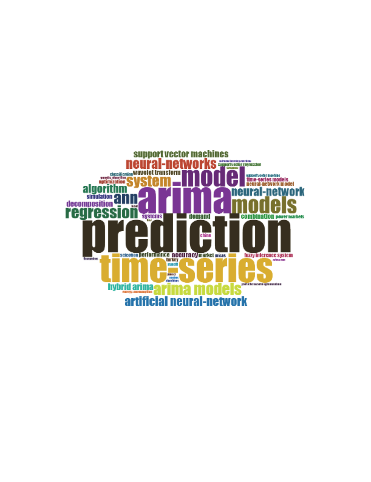In this survey, we have accomplished a survey on forecasting methods and the frequencies of the words used in Web of Science database. There are approximately 700 research works published and indexed in this database and Fig. 2 demonstrates the frequencis of the words used in research areas that use forecasting. Fig. 2. 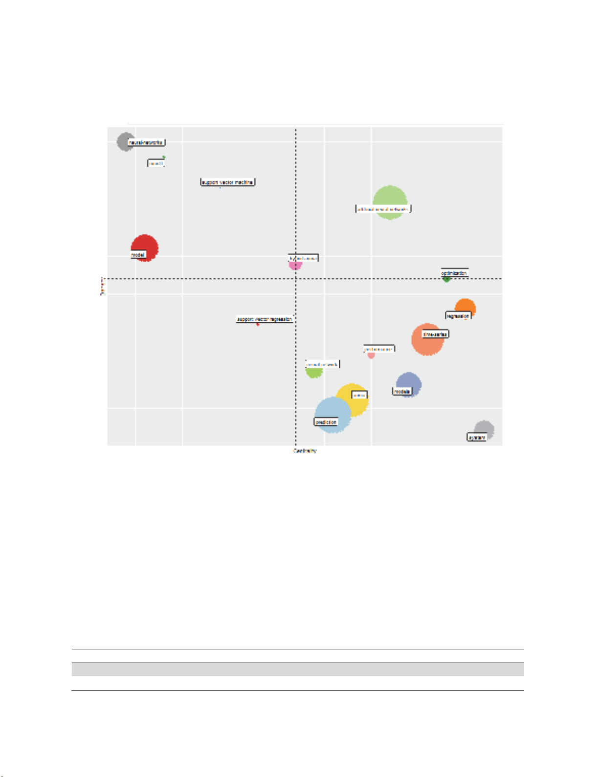The frequency of the keywords used in research topics with ARIMA and ANN According to Fig. 2, ANN and ARIMA have been extensively used in forecasting techniques. When co-word analysis is implemented for scientometrics purposes, we apply clusters of keywords and their interconnections and the clusters are addressed as themes. Each theme obtained here is specified in terms of two perspectives; namely “density” and “centrality” and some basic statistics for density and centrality are implemented for classification of the themes into various groups. In a theme, the keywords and their intercorrelations draw a network graph, called a “thematic network” where “centrality” is considered as the horizontal axis and “density” is taken into account as the vertical axis. In a network, if there is a big correlation from one node with other nodes, we consdier a higher centrality for it and it is considered as an important part in the network. Centrality is thus implemented to measure the correction degree among various topics. Thematic map is a kind of plot which makes it possible to analyze themes based on the quadrant in which they are placed. Themes in the upper-right quadrant are both well developed and important for the structuring of a research field such as “big data” and “big data analytics”. Themes in the upper-left quadrant have well developed internal ties but unimportant external ties and so are of only marginal importance for the field such as “social network”. Themes in
T. Alam / Decision Science Letters 8 (2019) 253 the lower-left quadrant are both “weakly developed and marginal”, mainly representing either emerging or disappearing. Themes in the lower-right quadrant are “important for a research field but are not developed”, so this quadrant groups transversal and general, basic themes such as “ARIMA” and “ANN” (See Fig. 3) (Esfahani et al., 2019; Salimi et al., 2019; Alavi et al., 2019; Gilani et al., 2019; Pourkhani et al., 2019; Tayebi et al., 2019; Javid et al., 2019). Fig. 3. Thematic Map Next, we present the results of the implementation of ARIMA and ANN methods. 3. Result and Findings 3.1.Data The data regarding the total annual exports and imports of the Kngdom was collected from Saudi Arabian Monetary Authority (SAMA). The information were on yearly basis and in Saudi Arabian Riyal (SAR) from years 1968 to 2017. The summary statistics for exports and imports data of the Kingdom are given below in the Table 3 by using Software XLSAT. Table 3 Summary Statistics of Export and Imports of the Kingdom Variable Observations Minimum Maximum Mean Std. deviation Exports 50 9118.000 1456502.000 384270.267 407367.661 Imports 50 2578.000 655033.364 181662.394 189268.157
254 3.2. Models for exports It is evident from the Fig. 4 and Fig. 5 that the exports of the Kingdom were gradually increasing and decreasing over time up till the year 2009 and after that they were continually increasing up to the year 2012. Also, it is evident from the figures that exports had a decreasing trend after 2012 up to 2016. After that, they were gradually increasing. ARIMA (Exports) 1600000 1400000 1200000 Exports 1000000 800000 600000 400000 200000 0 1960 1970 1980 1990 2000 2010 2020 2030 Year Exports ARIMA (Exports) Prediction Lower bound (95%) Upper bound (95%) Fig. 4. The results of Export using Neural Network Fig. 5. The results of of Export using ARIMA (1, 1, 2) 1 0.8 0.6 0.4 Autocorrelation 0.2 0 0 1 2 3 4 5 6 7 8 9 10 11 12 13 14 15 16 17 ‐0.2 ‐0.4 ‐0.6 ‐0.8 ‐1 Lag Fig. 6. Plot of ACF of Exports Fig. 6 shows that the autocorrelations were positive, strong and deteriorated slowly, which indicates that there were possible shifts in both the mean and the variability over time for this series. It means the arithmetic mean may be edging upwards, and the variability may be increasing and after that for time being edging downwards. 3.2.1 Prediction of the export ANN and ARIMA models are used to create the predictions for future values of the time series by using the XLSTAT package. From the Table 4, it is observed that the best prediction is provided by ANN and then ARIMA (1, 1, 2). Thus, we conclud that ANN model predicted the exports more efficiently than ARIMA models did.
T. Alam / Decision Science Letters 8 (2019) 255 Table 4 Prediction of Export of the Kingdom using different model Year Actual Value Predicted Value for Export (in million SAR) of Export ARIMA(1,0,0) ARIMA(0,1,1) ARIMA(1,1,2) ANN 2015 763313.06 1227127.829 1280858.878 1196259.604 767425.7889 2016 688423 739801.554 700605.619 679106.385 673640.1108 2017 831881.29 669726.153 703692.124 752574.815 842459.3463 2018 803961.547 851660.629 868907.714 1062343.541 2019 777836.759 851660.629 875109.992 1113639.628 2020 753391.526 851660.629 879892.482 952126.2365 RMSE 143006.113 143237.4797 134996.6626 46122.74 From Fig. 7, we concluded that the plot gives us an observed and predicted exports values for the years 1968 to 2017, as well as, for the next 3 years forecasted values of exports using ANN, ARIMA (1, 0, 0), ARIMA (0, 1, 0) and ARIMA (1, 1, 2) models. Predicted Value for Export (in million SAR) 1500000 Year ARIMA(1,0,0) 1000000 ARIMA(0,1,1) 500000 ARIMA(1,1,2) ANN 0 1 2 3 4 5 6 Fig. 7. Predicted Value for Export (in million SAR) 3.3.Models for Imports From the Fig. 8 and Fig. 9, it is concluded that the imports of the kingdom is also increasing and decreasing slowly over time up till year 2010 and after that it was continuously increasing up to year 2015. Also, it is evident from the above figures that imports are decreasing after 2015 up to 2017. After that, they are gradually increasing. Fig. 10 shows that the autocorrelations are strong, positive and deteriorating slowly which also indicates that there are possible shifts in both the mean and the variability over time for this series and the trend can be removed by differencing once or twice.
256 ARIMA (Imports) 700000 600000 500000 Imports 400000 300000 200000 100000 0 1960 1970 1980 1990 2000 2010 2020 2030 Year Imports ARIMA (Imports) Prediction Lower bound (95%) Upper bound (95%) Fig. 8. Graph of Import using Neural Network Fig. 9. Graph of Import using ARIMA (1, 1, 2) AutocorrelogramImports 1 0.8 0.6 Autocorrelation 0.4 0.2 0 ‐0.2 0 1 2 3 4 5 6 7 8 9 10 11 12 13 14 15 16 17 ‐0.4 ‐0.6 ‐0.8 ‐1 Lag Fig. 10. Plot of ACF of Exports 4. Prediction of Import From the Table 5, it is observed that the best prediction is provided by ANN followed by the arima model; ARIMA (0, 1, 1). Table 5 Prediction of Imports of the Kingdom using different model Year Actual Value of Predicted Value for Import (in million SAR) Import ARIMA(1,0.0) ARIMA(0,1,1) ARIMA(1,1,2) ANN 2015 655033.36 646286.769 664170.379 653917.967 642765.8139 2016 525636.01 649401.771 662035.706 651181.601 534745.5422 2017 504446.62 521740.477 486327.678 482240.964 498263.4603 2018 500835.375 511040.068 509805.874 500090.5623 2019 497272.583 511040.068 506271.174 499391.2118 2020 493757.591 511040.068 503003.332 510767.219 RMSE 37588.68409 34054.36786 33330.08092 15956 It is evident from the Fig. 11 that the plot could give us an observed and predicted imports values for the years 1968 to 2017, as well as for the next 3 years forecasted values of imports using ANN, ARIMA (1, 0, 0), ARIMA (0, 1, 0) and ARIMA (1, 1, 2) models.
T. Alam / Decision Science Letters 8 (2019) 257 Predicted Value for Import (in million SAR) 700000 600000 Year 500000 ARIMA(1,0.0) 400000 ARIMA(0,1,1) 300000 ARIMA(1,1,2) 200000 ANN 100000 0 1 2 3 4 5 6 Fig. 11. Predicted Value for Export (in million SAR) 5. Residual Analytic for ANN and ARIMA (1, 1, 2) It is evident from the Figs. 12-15, the residuals of the exports and imports of the models show analytic plots that are useful in making decision. From the aforementioned figures, we can say that the time series plot of the residuals model allow us to look for trends in the residuals. It is clear from the time series plot shown in the Figs. 12-15 that the series of residuals are a stationary series. Residuals 400000 300000 200000 100000 Residual 0 ‐100000 ‐200000 ‐300000 ‐400000 ‐500000 Year Fig. 12. Residual graph of export using neural Fig. 13. Residual Graph of Export using ARIMA (1, 1, 2) network Residuals 100000 50000 Residual 0 ‐50000 ‐100000 ‐150000 Year Fig. 14. Residual Graph of Import using Neural Fig. 13. Residual Graph of Import using ARIMA (1, 1, 2) Network
258 6. Conclusion In this paper, we have presented a comprehensive review on the applications of two models; namely artificial neural network (ANN) and ARIMA models for the purpose of forecasting. We have also mentioned that the historical review has shown a significant progress made in the field of ANN. Now, we can say that today is an epoch of evolution for neural network tools and techniques. An ARIMA model is one of the best techniques for predicting the level of any time series data with any pattern of change and is suitable for at least 50 observations. The primary objective of the study was to predict the total annual exports and imports of the Kingdom of Saudi Arabia. It has been evident from the analysis that ANN, ARIMA (0,1 ,1) and ARIMA (1,1,2) were the most appropriate models for forecasting the total annual exports and imports of the Kingdom of Saudi Arabia. The forecasted values of total annual exports and imports of the Kingdom will be 952126.2365 (in million SAR) and 510767.219 (in million SAR) respectively for the year 2020, which would be fluctuating as compared with 2014-15. References Alavi, S., Mehdinezhad, I & Kahshidinia, B. (2019). A trend study on the impact of social media on advertisement.International Journal of Data and Network Science, 3(3), 185-200. Ardakani, F. J., & Ardehali, M. M. (2014a). Long-term electrical energy consumption forecasting for developing and developed economies based on different optimized models and historical data types. Energy, 65, 452-461. Ardakani, F. J., & Ardehali, M. M. (2014b). Novel effects of demand side management data on accuracy of electrical energy consumption modeling and long-term forecasting. Energy conversion and management, 78, 745-752. Aydin, G., Jang, H., & Topal, E. (2016). Energy consumption modeling using artificial neural networks: The case of the world’s highest consumers. Energy Sources, Part B: Economics, Planning, and Policy, 11(3), 212-219. Box, G. E., Jenkins, G. M., Reinsel, G. C., & Ljung, G. M. (2015). Time series analysis: forecasting and control. John Wiley & Sons. Chamberlain, G. (1982). Multivariate regression models for panel data. Journal of Econometrics, 18(1), 5-46. Chang, C. C., & Lin, C. J. (2011). LIBSVM: a library for support vector machines. ACM Transactions on Intelligent Systems and Technology (TIST), 2(3), 27. Deng, J. (2010, August). Energy demand estimation of China using artificial neural network. In Business Intelligence and Financial Engineering (BIFE), 2010 Third International Conference on (pp. 32-34). IEEE. Esfahani, H., Tavasoli, K & Jabbarzadeh, A. (2019). Big data and social media: A scientometrics analysis.International Journal of Data and Network Science, 3(3), 145-164. Feng, Y., Liu, J., & He, Y. (2013). Chaos-based dynamic population firefly algorithm. Journal of Computer Applications, 33(3), 796-799. Gaida, A. J., Grigorian, T. G., Zarichuk, E. A., & Koshkin, K. V. (2017, May). The decision making mechanisms in sea container traffic management. In Electrical and Computer Engineering (UKRCON), 2017 IEEE First Ukraine Conference on (pp. 935-938). IEEE. Gilani, E., Salimi, D., Jouyandeh, M., Tavasoli, K & Wong, W. (2019). A trend study on the impact of social media in decision making.International Journal of Data and Network Science, 3(3), 201-222. Hsu, C. W., & Lin, C. J. (2002). A comparison of methods for multiclass support vector machines. IEEE transactions on Neural Networks, 13(2), 415-425. Javid, E., Nazari, M & Ghaeli, M. (2019). Social media and e-commerce: A scientometrics analysis. International Journal of Data and Network Science, 3(3), 269-290.
T. Alam / Decision Science Letters 8 (2019) 259 Joachims, T. (1998, April). Text categorization with support vector machines: Learning with many relevant features. In European conference on machine learning (pp. 137-142). Springer, Berlin, Heidelberg. Kankal, M., & Uzlu, E. (2017). Neural network approach with teaching–learning-based optimization for modeling and forecasting long-term electric energy demand in Turkey. Neural Computing and Applications, 28(1), 737-747. Kavaklioglu, K., Ceylan, H., Ozturk, H. K., & Canyurt, O. E. (2009). Modeling and prediction of Turkey’s electricity consumption using artificial neural networks. Energy Conversion and Management, 50(11), 2719-2727. Kazem, A., Sharifi, E., Hussain, F. K., Saberi, M., & Hussain, O. K. (2013). Support vector regression with chaos-based firefly algorithm for stock market price forecasting. Applied Soft Computing, 13(2), 947-958. Kendall, M. G (1995). Time series. Griffin and Co ltd, London. Khashei, M., & Bijari, M. (2010). An artificial neural network (p, d, q) model for timeseries forecasting. Expert Systems with Applications, 37(1), 479-489. Khashei, M., & Bijari, M. (2011). A novel hybridization of artificial neural networks and ARIMA models for time series forecasting. Applied Soft Computing, 11(2), 2664-2675. Kotur, D., & Žarković, M. (2016, September). Neural network models for electricity prices and loads short and long-term prediction. In Environment Friendly Energies and Applications (EFEA), 2016 4th International Symposium on (pp. 1-5). IEEE. Li, A., Liang, S., Wang, A., & Qin, J. (2007). Estimating crop yield from multi-temporal satellite data using multivariate regression and neural network techniques. Photogrammetric Engineering & Remote Sensing, 73(10), 1149-1157. Liu, D., Niu, D., Wang, H., & Fan, L. (2014). Short-term wind speed forecasting using wavelet transform and support vector machines optimized by genetic algorithm. Renewable Energy, 62, 592- 597. Liu, B., Fu, C., Bielefield, A., & Liu, Y. Q. (2017). Forecasting of Chinese primary energy consumption in 2021 with GRU artificial neural network. Energies, 10(10), 1453. Ljung, G. M., & Box, G. E. (1978). On a measure of lack of fit in time series models. Biometrika, 65(2), 297-303. Mollaiy-Berneti, S. (2015). Developing energy forecasting model using hybrid artificial intelligence method. Journal of Central South University, 22(8), 3026-3032. Montanari, A., Rosso, R., & Taqqu, M. S. (1997). Fractionally differenced ARIMA models applied to hydrologic time series: Identification, estimation, and simulation. Water Resources Research, 33(5), 1035-1044. Olajide, J. T., Ayansola, O. A., Odusina, M. T., & Oyenuga, I. F. (2012). Forecasting the Inflation Rate in Nigeria: Box Jenkins Approach. IOSR Journal of Mathematics (IOSR-JM), 3(5), 15-19. Olgun, M. O., Ozdemir, G., & Aydemir, E. (2012). Forecasting of Turkey's natural gas demand using artifical neural networks and support vector machines. Energy Education Science and Technology Part A: Energy and Research, 30(1), 15-20. Panda, S. S., Ames, D. P., & Panigrahi, S. (2010). Application of vegetation indices for agricultural crop yield prediction using neural network techniques. Remote Sensing, 2(3), 673-696. Pedro, H. T., & Coimbra, C. F. (2012). Assessment of forecasting techniques for solar power production with no exogenous inputs. Solar Energy, 86(7), 2017-2028. Pourkhani, A., Abdipour, K., Baher, B & Moslehpour, M. (2019). The impact of social media in business growth and performance: A scientometrics analysis. International Journal of Data and Network Science, 3(3), 223-244. Salimi, D., Tavasoli, K., Gilani, E., Jouyandeh, M & Sadjadi, S. (2019). The impact of social media on marketing using bibliometrics analysis. International Journal of Data and Network Science, 3(3), 165-184. Reikard, G. (2009). Predicting solar radiation at high resolutions: A comparison of time series forecasts. Solar Energy, 83(3), 342-349.
260 Sözen, A., Isikan, O., Menlik, T., & Arcaklioglu, E. (2011). The forecasting of net electricity consumption of the consumer groups in Turkey. Energy Sources, Part B: Economics, Planning, and Policy, 6(1), 20-46. Sokolov-Mladenović, S., Milovančević, M., Mladenović, I., & Alizamir, M. (2016). Economic growth forecasting by artificial neural network with extreme learning machine based on trade, import and export parameters. Computers in Human Behavior, 65, 43-45. Tayebi, S., Manesh, S., Khalili, M & Sadi-Nezhad, S. (2019). The role of information systems in communication through social media. International Journal of Data and Network Science, 3(3), 245-268. Tektaş, M. (2010). Weather forecasting using ANFIS and ARIMA models. Environmental Research, Engineering and Management, 51(1), 5-10. Tsai, F. M., & Huang, L. J. (2017). Using artificial neural networks to predict container flows between the major ports of Asia. International Journal of Production Research, 55(17), 5001-5010. Uddin, J. (2009). Time series behavior of imports and exports of bangladesh: Evidence from cointegration analysis and error correction model. International Journal of Economics and Finance, 1(2), 156. Udny Yule, G. (1927). On a method of investigating periodicities in disturbed series, with special reference to Wolfer's sunspot numbers. Philosophical Transactions of the Royal Society of London Series A, 226, 267-298. Valipour, M., Banihabib, M. E., & Behbahani, S. M. R. (2013). Comparison of the ARMA, ARIMA, and the autoregressive artificial neural network models in forecasting the monthly inflow of Dez dam reservoir. Journal of hydrology, 476, 433-441. Walker, G. T. (1931). On periodicity in series of related terms. Proceedings of the Royal Society of London. Series A, Containing Papers of a Mathematical and Physical Character, 131(818), 518- 532. Wang, W. C., Chau, K. W., Xu, D. M., & Chen, X. Y. (2015). Improving forecasting accuracy of annual runoff time series using ARIMA based on EEMD decomposition. Water Resources Management, 29(8), 2655-2675. Wold, H. A. (1938). Study in the analysis of stationary time series, Stockholm. Department of Mathematics State University of New York Stony Brook, NY, 11794. Zeng, Y. R., Zeng, Y., Choi, B., & Wang, L. (2017). Multifactor-influenced energy consumption forecasting using enhanced back-propagation neural network. Energy, 127, 381-396. https://atlas.media.mit.edu/en/profile/country/sau/ http://www.sama.gov.sa/en © 2019 by the authors; licensee Growing Science, Canada. This is an open access article distributed under the terms and conditions of the Creative Commons Attribution (CC-BY) license (http://creativecommons.org/licenses/by/4.0/).