
http://www.iaeme.com/IJMET/index.asp 487 editor@iaeme.com
International Journal of Mechanical Engineering and Technology (IJMET)
Volume 10, Issue 03, March 2019, pp. 487-495. Article ID: IJMET_10_03_051
Available online at http://www.iaeme.com/ijmet/issues.asp?JType=IJMET&VType=10&IType=3
ISSN Print: 0976-6340 and ISSN Online: 0976-6359
© IAEME Publication Scopus Indexed
APPLICATION OF GREY RELATIONAL
ANALYSIS FOR MULTI VARIABLE
OPTIMIZATION OF PROCESS PARAMETERS
IN DRILLING OF POLYMER BASED GLASS
FIBER REINFORCED COMPOSITE
Dr. Murthy BRN and Dr. Rajendra Beedu*
1Department of Mechanical and Manufacturing, Manipal Institute of Technology, Manipal.
Karnataka, India.
*Corresponding Author
ABSTRACT
The present work deals with a simple approach which predicts the optimum setting
of process parameters of drilling operation on Polymer Based Glass Fiber (PBGF)
composite. The process parameters selected are drill angle (DA), Drill diameter (DD),
Material Thickness (MT), Speed (N) and Feed (f). The output parameters are Thrust,
Torque, Surface Roughness and Delamination. Three levels of each input parameters
are considered. Taguchi’s L27 array is used to set the process parameters. Gray
relational analysis (GRA) is used to find the optimum value of process parameters.
Conduction of ANOVA on GRA shown the significance of each factor on the process
output. A conformation test conducted revealed that the setting of parameters ensures
optimum output.
Keywords: Drilling, PBGF composite, orthogonal array, Gray relational analysis.
Cite this Article: Dr. Murthy BRN and Dr. Rajendra Beedu, Application of Grey
Relational Analysis for Multi Variable Optimization of Process Parameters in Drilling
of Polymer Based Glass Fiber Reinforced Composite, International Journal of
Mechanical Engineering and Technology, 10(3), 2019, pp. 487-495
http://www.iaeme.com/IJMET/issues.asp?JType=IJMET&VType=10&IType=3
1. INTRODUCTION
The use of Polymer based glass fiber (PBGF) is extending beyond the initial applications in
aerospace and military fields, driven by the advances in manufacturing technologies which
has made the production process more cost effective. PBGF composite materials offer
excellent mechanical properties, while being much more lightweight than the metallic alloys.
As PBGF composite parts are usually integrated in a mechanical assembly, drilling is the
most common encountered machining process in the production of such parts. Drilling is

Dr. Murthy BRN and Dr. Rajendra Beedu
http://www.iaeme.com/IJMET/index.asp 488 editor@iaeme.com
carried out during the final stages of the manufacturing process in order to create holes for
fabrication.
Excessive tool wear and delamination are the two major problems highlighted in the
drilling process of the PBGF composites. The excessive tool wear makes the drilling process
of the fiber reinforced composites very expensive, only a limited number of holes can be
drilled with one particular drill. Delamination is the one of the main reasons which is leading
rejection of composite parts in the larger quantity.
Most of the researchers are focusing on characterization of PBGF composite. But the main
problem occurs in drilling holes for the purpose of assembly. The components made by PBGF
may fail due to delamination and rough surface, excess thrust force and torque associated with
speed. Hence optimization of process parameters is essential to reduce the damage occurs
during drilling process in order to reduce the rejection of composite components. Literature
review reveals that many researchers are made attempts to optimize the process parameters to
achieve the good quality holes by minimizing the thrust force, torque, surface roughness and
delamination factor. Palanikumar [1] used Taguchi and response surface methodology to
optimese the process parameters to achieve the minimum surface roughness. Enemuoh et al.
[2] proposed an approach of combining Taguchi’s technique and multi-objective optimization
criterion to select cutting parameter for damage-free drilling in carbon fiber-reinforced epoxy
composite materials. Ghani et al. [3] developed a new approach using Taguchi’s method to
optimize the cutting parameters in end milling of AISI H1312. K. Karthik et al. [4] optimized
the process parameters to minimize the delamination on the drilling of GFRP composites
using HSS drill bits. Lewlyn L. R. Rodrigues et al. [5] optimized the process parameters in the
drilling of CFRP composites to reduce the surface roughness using Taguchi and RSM
methods. S Aril et al. [6] did the optimization in drilling of GFRP composites using HSS
drills to achieve the lower delamination. They used an optimization algorithm using simulated
annealing with a performance index for this purpose. In this way numerous numbers of
researchers used various methods to optimize the process parameters to obtain the desired
outputs [7-9]. In the literature review we noticed that they did optimization for one output
parameter at a time. But in this present work we tried to develop the optimization for four
output parameters at a time. Production of acceptable components with minimum failure is
the main purpose of setting proper process parameters.
2. FABRICATION OF COMPOSITE
The glass fiber reinforced resin composite required for testing was manufactured through
hand layup method. The glass fibers are reinforced in general purpose resin matrix. Chopped
glass mat is used for reinforcement which is presented in Figure 1a and the prepared
composite sheet in Figure 1b.
Figure 1a Chopped glass mat Figure 1b Prepared composite specimen
2.1. Selection of Levels of Drilling Parameters
Application of Grey Relational Analysis for Multi Variable Optimization of Process Parameters in
Drilling of Polymer Based Glass Fiber Reinforced Composite
http://www.iaeme.com/IJMET/index.asp 489 editor@iaeme.com
The input drilling parameters are selected as per the available literature survey information,
solid carbide drill bits are used because of their low wear characteristics. All five parameters
and their levels chosen for the present work are shown in Table1.
Table 1 Levels of process parameters
Parameters
Drill angle
(DA) degrees
(A)
Drill Diameter
(DD) mm
(B)
Material
Thickness (MT
mm) (C)
Speed (N) RPM
(D)
Feed (f) m/min
(E)
Level 1
90
6
8
900
75
Level 2
103
8
10
1200
110
Level 3
118
10
12
1500
150
2.2. Selection of process parameters for each trial and measurement of output
parameters
The process parameters are selected according to Taguchi’s L27 orthogonal array. This array
ensures minimum number of experiments to be conducted with nearly accurate solution. The
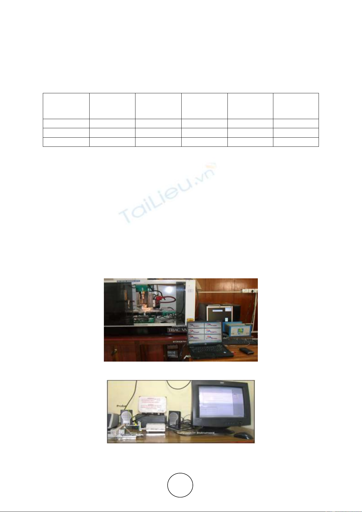
drilling experiments were conducted on a CNC machine which is capable of drilling accurate
and precise holes. WC tool is used. The experimentation set up to drill the holes and to
measure the thrust and torque produced during the machining is process is shown in Figure 2.
The output parameters are measured and listed as shown in table 2. The thrust force and
torque are measured using Kistler dynamometer, surface roughness using Taylor Hobson
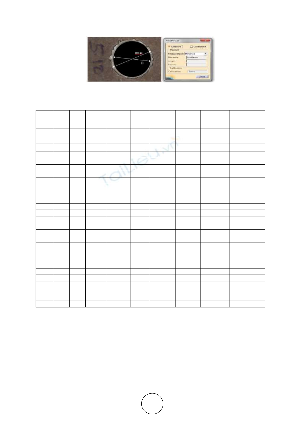
Surtronic 3+ roughness measurement instrument and delamination factor was estimated by
taking the images of the drilled with the help of high resolution scanner and measuring the
dimensions of scanned images by using CATIA software. Arrangement made to measure
surface roughness and delamination is presented in figures 3 and 4. The measured data is
illustrated in Table 2.
Figure 2 Experimental set-up to drill the holes and to measure thrust and torque.
Figure 3 Measurement of surface roughness
Dr. Murthy BRN and Dr. Rajendra Beedu
http://www.iaeme.com/IJMET/index.asp 490 editor@iaeme.com
Figure 4 Measurement of delamination factor
Table 2 L27 orthogonal array with factors and responses
Trial
No
A
B
C
D
E
Thrust (N)
Torque
(N-mm)
Surface
Roughness
µm
Delamination
1
1
1
1
1
1
29.67
16.32
2.99
1.06
2
1
1
1
1
2
36.20
18.04
3.11
1.07
3
1
1
1
1
3
38.20
20.46
3.29
1.08
4
1
2
2
2
1
31.65
30.04
3.20
1.09
5
1
2
2
2
2
33.99
30.23
3.23
1.10
6
1
2
2
2
3
34.16
24.66
3.24
1.11
7
1
3
3
3
1
36.04
27.64
3.35
1.11
8
1
3
3
3
2
37.86
28.45
3.37
1.12
9
1
3
3
3
3
38.04
34.23
3.40
1.13
10
2
1
2
3
1
34.98
14.66
3.20
1.09
11
2
1
2
3
2
36.38
14.02
3.30
1.10
12
2
1
2
3
3
36.77
14.34
3.33
1.16
13
2
2
3
1
1
44.27
26.98
3.40
1.11
14
2
2
3
1
2
45.83
27.09
3.42
1.12
15
2
2
3
1
3
46.98
30.65
3.48
1.13
16
2
3
1
2
1
40.71
26.92
3.20
1.07
17
2
3
1
2
2
40.29
29.98
3.30
1.10
18
2
3
1
2
3
40.46
24.97
3.31
1.10
19
3
1
3
2
1
42.98
17.46
3.57
1.11
20
3
1
3
2
2
43.36
18.02
3.58
1.12
21
3
1
3
2
3
45.36
19.18
3.59
1.13
22
3
2
1
3
1
40.46
17.70
3.25
1.09
23
3
2
1
3
2
41.32
17.39
3.30
1.11
24
3
2
1
3
3
42.56
17.67
3.11
1.14
25
3
3
2
1
1
58.36
41.01
3.37
1.10
26
3
3
2
1
2
59.38
41.46
3.38
1.11
27
3
3
2
1
3
59.98
41.96
3.39
1.11
Number of replication of each factor is 1 (k=1). The responses are measured in different
units and has different ranges. For multi-response optimization, the results are brought in the
range 0 to 1 by the process called normalization. Normalisation scales down the responses in
an acceptable range for further operation.
2.3. Normalisation
The response parameter is of two types i.e, beneficiary (maximum the better) and non-
benificiery (minimum the better). For beneficiary attribute j, the normalized parameter of the
trial i and replication k is given by
and for non beneficiary attribute

Application of Grey Relational Analysis for Multi Variable Optimization of Process Parameters in
Drilling of Polymer Based Glass Fiber Reinforced Composite
http://www.iaeme.com/IJMET/index.asp 491 editor@iaeme.com
where k is the replication. In this paper all response parameters are
non beneficiary type. The actual response X ijk is modified to X’ijk which ranges from 0 to 1.
The maximum value of normalized response, irrespective of response parameter is taken as
reference value R.
R = 1.
2.4. Calculation of difference value
The difference value is calculated by, | |. The difference values arrange the
output response in the ascending order for non-beneficiary attribute. These value is used to
calculate Gray relational Coefficient
2.5. Calculation of Grey Relational Coefficient GRCijk
The Grey Relational Coefficient is calculated by the formula,
where ξ is the distinguishing coefficient ranging from 0 to 1. Generally, ξ is taken as 0.5.
2.6. Calculation of Grey Relational Grade
The average of GRC in each row is known as Grey Relational Grade . The Grey
relational grade is given by the formula, ∑ ∑
where m is the number of
response parameters and n is the number of replications (n=1).
The calculated GRG is shown in Table 3
Table 3 Orthogonal Array with Gray Relational Grades.
Trial No
A
B
C
D
E
GRG
1
1
1
1
1
1
0.67
2
1
1
1
1
2
0.58
3
1
1
1
1
3
0.50
4
1
2
2
2
1
0.53
5
1
2
2
2
2
0.51
6
1
2
2
2
3
0.47
7
1
3
3
3
1
0.46
8
1
3
3
3
2
0.45
9
1
3
3
3
3
0.47
10
2
1
2
3
1
0.48
11
2
1
2
3
2
0.44
12
2
1
2
3
3
0.38
13
2
2
3
1
1
0.48
14
2
2
3
1
2
0.47
15
2
2
3
1
3
0.47
16
2
3
1
2
1
0.58
17
2
3
1
2
2
0.51
18
2
3
1
2
3
0.48
19
3
1
3
2
1
0.42
20
3
1
3
2
2
0.41


![Bài tập tối ưu trong gia công cắt gọt [kèm lời giải chi tiết]](https://cdn.tailieu.vn/images/document/thumbnail/2025/20251129/dinhd8055/135x160/26351764558606.jpg)