Predicting bike-sharing demand using random forest

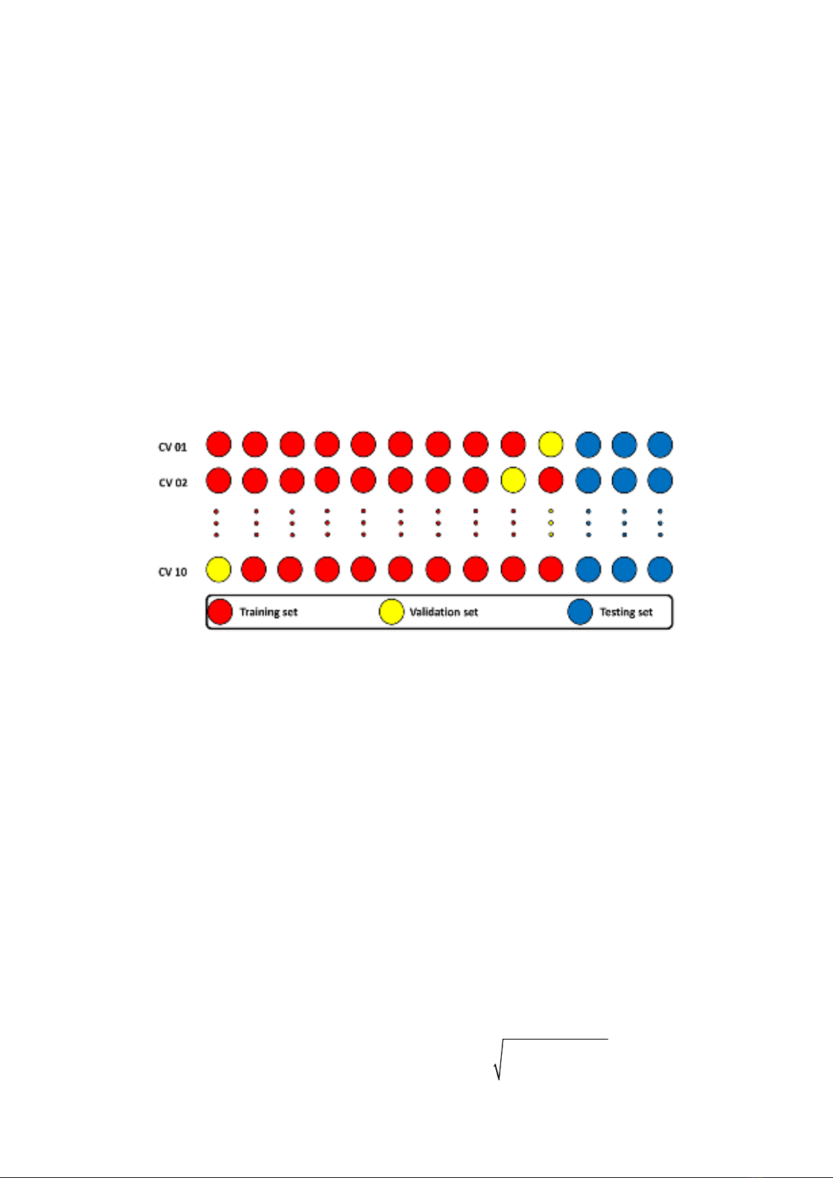
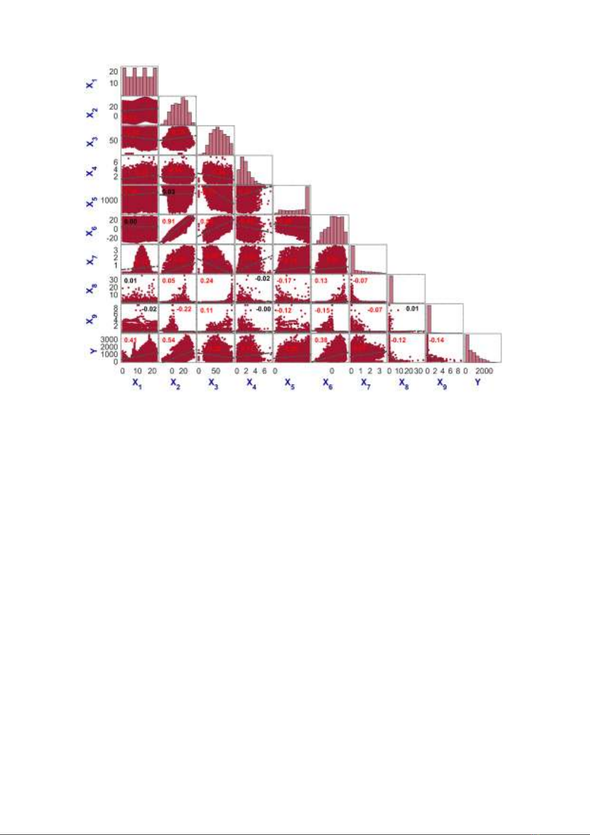
This article uses Random Forest (RF) and k-fold cross-validation to predict the hourly count of rental bikes (cnt/h) in the city of Seoul (Korea) using information related to rental hour, temperature, humidity, wind speed, visibility, dewpoint, solar radiation, snowfall, and rainfall.