The Economic Theory of Annuities by Eytan Sheshinski_4

Chia sẻ: Thao Thao | Ngày: | Loại File: PDF | Số trang:19

Thêm vào BST

Báo xấu

75
lượt xem 9
download

Download Vui lòng tải xuống để xem tài liệu đầy đủ

Tham khảo tài liệu 'the economic theory of annuities by eytan sheshinski_4', tài chính - ngân hàng, ngân hàng - tín dụng phục vụ nhu cầu học tập, nghiên cứu và làm việc hiệu quả

Chủ đề:

Bình luận(0) Đăng nhập để gửi bình luận!

Lưu

Nội dung Text: The Economic Theory of Annuities by Eytan Sheshinski_4

August 3, 2007 Time: 04:26pm chapter10.tex 80 • Chapter 10 particular, the individual typically has some inﬂuence on the outcome. Thus, the probability q, which was taken as given, may be regarded, to some extent at least, as inﬂuenced by individual decisions that involve costs and efforts. The potential conﬂict that this type of moral hazard raises between social welfare and individual interests is very clear in this ∗ ∗ context. Since V1 < V2 , an increase in q decreases the ﬁrst-best expected ˆ ˆ utility. On the other hand, in a competitive equilibrium, V1 > V2 , and hence an increase in q may be desirable.
August 20, 2007 Time: 05:49pm chapter09.tex CHAPTER 9 Pooling Equilibrium and Adverse Selection 9.1 Introduction For a competitive annuity market with long-term annuities to be efﬁcient, it must be assumed that individuals can be identiﬁed by their risk classes. We now wish to explore the existence of an equilibrium in which the individuals’ risk classes are unknown and cannot be revealed by their actions. This is called a pooling equilibrium. Annuities are offered in a pooling equilibrium at the same price to all individuals (assuming that nonlinear prices, which require exclusivity, as in Rothschild and Stiglitz (1979), are not feasible). Consequently, the equilibrium price of annuities is equal to the average longevity of the annuitants, weighted by the equilibrium amounts purchased by different risk classes. This result has two important implications. One, the amount of annuities purchased by individuals with high longevity is larger than in a separating, efﬁcient equilibrium, and the opposite holds for individuals with low longevities. This is termed adverse selection. Two, adverse selection causes the prices of annuities to exceed the present values of expected average actuarial payouts. The empirical importance of adverse selection is widely debated (see, for example, Chiapori and Salanie (2000), though its presence is visible. For example, from the data in Brown et al. (2001), one can derive survival rates for males and females born in 1935, distinguish- ing between the overall population average rates and the rates appli- cable to annuitants, that is, those who purchase private annuities. As ﬁgures 9.1(a) and (b) clearly display, at all ages annuitants, whether males or females, have higher survival rates than the population average rates (table 9A.1 in the appendix provides the underlying data). Adverse selection seems somewhat smaller among females, perhaps because of the smaller variance in female survival rates across different occupations and educational groups. Adverse selection may be reﬂected not only in the amounts of annuities purchased by different risk classes but also in the selection of different insurance instruments, such as different types of annuities. We explore this important issue in chapter 11.
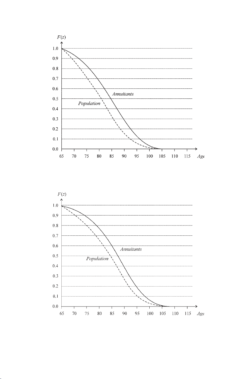
August 20, 2007 Time: 05:49pm chapter09.tex (a) Z Figure 9.1(a). Male survival functions (1935 cohort). (Source: Brown et al. 2001, table 1.1). (b) Z Figure 9.1(b). Female survival functions (1935 cohort). (Source: Brown et al. 2001, table 1.1). 68
August 20, 2007 Time: 05:49pm chapter09.tex Pooling Equilibrium • 69 9.2 General Model We continue to denote the ﬂow of returns on long-term annuities purchased prior to age M by r (z), M ≤ z ≤ T . The dynamic budget constraint of a risk-class-i individual, i = 1, 2, is now a i (z) = r p (z)ai (z) + w (z) − ci (z) + r (z)a ( M), M ≤ z ≤ T, ˙ (9.1) where a i (z) are annuities purchased or sold (with ai ( M) = 0) and r p (z) ˙ is the rate of return in the (pooled) annuity market for age-z individuals, M ≤ z ≤ T. For any consumption path, the demand for annuities is, by (9.1), z z x ai (z) = exp exp − r p (x) dx r p (h) dh M M M ×(w (x) − ci (x) + r (x)a ( M)) dx , i = 1, 2. (9.2) Maximization of expected utility, T Fi (z)u(ci (z)) dz, i = 1, 2, (9.3) M subject to (9.1) yields optimum consumption, denoted ci (z), ˆ z 1 ci (z) = ci ( M) exp (r p (x) − ri (x)) dx , M ≤ z ≤ T, i = 1, 2 ˆ ˆ σ M (9.4) (where σ is evaluated at ci (x)). It is seen that ci (z) increases or decreases ˆ ˆ with age depending on the sign of r p (z) − ri (z). Optimum consumption at age M, ci ( M), is found from (9.2), setting ai (T ) = 0, T x exp − r p (h) dh (w (x) − ci (x) + r (x)a ( M)) dx = 0, i = 1, 2. ˆ M M (9.5) Substituting for ci (x), from (9.4), ˆ T x exp − Mr p (h) dh (w ( x) + r ( x)a ( M)) dx ci ( M) = , i = 1, 2. (9.6) M ˆ T x1 M σ ((1 − σ )r p (h) − ri (h)) dh d x exp M
August 20, 2007 Time: 05:49pm chapter09.tex 70 • Chapter 9 Since r1 (z) < r2 (z) for all z, M ≤ z ≤ T, it follows from (9.6) that c1 ( M) < c2 ( M). Inserting optimum consumption ci (x) into (9.2), we ˆ ˆ ˆ obtain the optimum demand for annuities, ai (z).ˆ ˙ ˙ Since a i ( M) = 0, it is seen from (9.1) that a1 ( M) > a2 ( M). In fact, it ˆ ˆ ˆ can be shown (see appendix) that a 1 (z) > a 2 (z) for all M < z < T. ˆ ˆ This is to be expected: At all ages, the stochastically dominant risk class, having higher longevity, holds more annuities compared to the risk class with lower longevity. We wish to examine whether there exists an equilibrium pooling rate of return, r p (z), that satisﬁes the aggregate resource constraint (zero expected proﬁts). Multiplying (9.1) by Fi (z) and integrating by parts, we obtain T Fi (z)(r p (z) − ri (z))ai (z) dz ˆ M T T = Fi (z)(w (z) − ci (z))dz + a M r (z) dz, i = 1, 2. ˆ (9.7) M M Multiplying (9.7) by p for i = 1 and by (1 − p) for i = 2, and adding, T [( pF1 (z)a 1 (z) + (1 − p) F2 (z)a 2 (z)) r p (z) ˆ ˆ M − ( pF1 (z)a 1 (z)r1 (z) + (1 − p) F2 (z)a2 (z)r2 (z))] dz ˆ ˆ T M =p F1 (z)(w (z) − c1 (z)) dz + (1 − p) F2 (z)(w (z) − c2 (z)) dz ˆ ˆ M T T + a ( M) ( pF1 (z) + (1 − p) F2 (z)) r (z) dz. (9.8) M Recall that pF1 (z)r1 (z) + (1 − p) F2 (z)r2 (z) r (z) = pF1 (z) + (1 − p) F2 (z) is the rate of return on annuities purchased prior to age M. Hence the last term on the right hand side of (9.8) is equal to F ( M)a ( M) = M 0 F (z)(w (z) − c) dz. Thus, the no-arbitrage condition in the pooled
August 20, 2007 Time: 05:49pm chapter09.tex Pooling Equilibrium • 71 market is satisﬁed if and only if the left hand side of (9.8) is equal to 0 for all z: r p (z) = γ (z)r1 (z) + (1 − γ (z))r2 (z), (9.9) where ˆ pF1 (z)a1 (z) γ (z) = . (9.10) pF1 (z)a1 (z) + (1 − p)a2 (z) ˆ ˆ The equilibrium pooling rate of return takes into account the amount of annuities purchased or sold by the two risk classes. Assuming that ai (z) > 0, i = 1, 2, r p (z) is seen to be a weighted average of r1 (z) and ˆ r2 (z): r1 (z) < r p (z) < r2 (z). In the appendix we discuss the conditions that ensure positive holdings of annuities by both risk classes. Comparing (9.9) and (9.10) with (8.25) and (8.26), it is seen that r p (z) < r (z) for all z, M < z < T. The pooling rate of return on annuities, reﬂecting adverse selection in the purchase of annuities in equilibrium, is lower than the rate of return on annuities purchased prior to the realization of different risk classes. Indeed, as described in the introduction to this chapter, Brown et al. (2001) compared mortality tables for annuitants to those for the general population for both males and females and found signiﬁcantly higher expected lifetimes for the former. In chapter 11 we shall explore another aspect of adverse selection, annuitants’ self-selection leading to sorting among different types of annuities according to equilibrium prices. 9.3 Example Assume that u(c) = ln c, F (z) = e−α z , 0 ≤ z ≤ M, Fi (z) = e−α M e−αi (z− M) , M ≤ z ≤ ∞, i = 1, 2, w (z) = w constant and let retirement age, R, be independent of risk class.1 Under these assumptions, (9.6) becomes ∞ x ci ( M) = α i exp − r p (h) dh (w (x) + r (x)a ( M)) dx, ˆ (9.11) M M where w (x) = w for M ≤ x ≤ R and w (x) = 0 for x > R. 1 Individuals have an inelastic inﬁnite labor disutility at R and zero disutility at ages z < R.
August 20, 2007 Time: 05:49pm chapter09.tex 72 • Chapter 9 M Figure 9.2. Demand for annuities in a pooling equilibrium. Demand for annuities, (9.2), is now z x x a i (z) = exp exp − r p (h) dh (w (x) + r (x)a ( M)) dx ˆ r p (x) dx M M M ∞ x − 1 − e−αi (z− M) exp − r p (h) dh (w (x) + r (x)a ( M)) dx. M M (9.12) Clearly, ai ( M) = ai (∞) = 0, i = 1, 2, and since α 1 < α 2 , it follows that a1 (z) > a2 (z) for all z > M. From (9.1), ˆ ˆ R x · a i ( M) = w 1 − α i exp − r p (h) dh d x + a ( M) ˆ M M ∞ x × r ( M) − α i exp − r p (h) dh r (x) dx , i = 1, 2. M M (9.13) Since r (x) decreases in x, (8.29), it is seen that if r p (x) > α 1 , then ˙ for i = 1, both terms in (9.13) are positive, and hence a1 ( M) > 0. ˆ From (9.12) it can then be inferred that a1 (z) > 0 with the shape in ˆ ﬁgure 9.2.
August 20, 2007 Time: 05:49pm chapter09.tex Pooling Equilibrium • 73 M Figure 9.3. Return on annuities in a pooling equilibrium. ˙ Additional conditions are required to ensure that a2 ( M) > 0, from ˆ which it follows that a2 (z) > 0, z ≥ M. Thus, the existence of a pool- ˆ ing equilibrium depends on parameter conﬁguration. When a2 (z) > 0 ˆ (ﬁgure 9.2), then r (z) = δ (z)α 1 + (1 − δ )α 2 > r p (z) = γ (z)α 1 + (1 − γ (z))α 2 because when a1 (z) > a2 (z), then (ﬁgure 9.3) ˆ ˆ pe−α1 (z− M) δ (z) = pe−α1 (z− M) + (1 − p)e−α2 (z− M) pe−α1 (z− M) a1 (z) ˆ > = γ (z). pe−α1 (z− M) a (z) + (1 − p)e−α2 (z− M) a2 (z) ˆ ˆ 1 What remains to be determined is the optimum a ( M), a ( M) = ˆ ˆ ((w − c)/α )(eα M − 1), or, equivalently, consumption prior to age M, c = ˆ ˆ w −α a ( M)/(eα M − 1). By (9.11), ci ( M), i = 1, 2, depend directly on a ( M). ˆ ˆ ˆ Maximizing expected utility (disregarding labor disutility), ∞ M e−α z ln c dz + pe−α M e−α1 (z− M) ln c1 (z) dz V= ˆ 0 M ∞ +(1 − p)e−α M e−α2 (z− M) ln c2 (z) dz, ˆ (9.14) M
August 20, 2007 Time: 05:49pm chapter09.tex 74 • Chapter 9 Figure 9.4. Amount of long-term annuities purchased early in life: ∞ x R x A = M exp − Mr p (h) dh r (x) dx/ M exp − Mr p (h) dh d x > 1 . with respect to a ( M), using (9.11), yields the ﬁrst-order condition for an interior solution that can be written, after some manipulations as eα M − 1 p p = + w (eα M − 1) − α a ( M) α1 α2   ∞ x   exp(− M r p (h) dh)r ( x) dx ×  M   x ∞ exp − r p (h) dh (w (x) + c(x)a ( M)) dx M M (9.15) The left-hand side of (9.15) increases with a ( M), while the right hand side decreases with a ( M) (ﬁgure 9.4).
August 20, 2007 Time: 05:49pm chapter09.tex Appendix A. Survival Rates for a 1935 Birth Cohort Table 9.A.1. Population Annuitants Age Male Female Male Female 65 0.978503 0.986735 0.989007 0.992983 66 0.955567 0.972336 0.977086 0.985266 67 0.931401 0.956873 0.964103 0.976922 68 0.906303 0.940484 0.949935 0.967886 69 0.880455 0.923244 0.934490 0.958116 70 0.853800 0.905086 0.917697 0.947530 71 0.826172 0.885875 0.899490 0.936004 72 0.797493 0.865541 0.879829 0.923386 73 0.767666 0.843998 0.858678 0.909496 74 0.736589 0.821157 0.835989 0.894166 75 0.704187 0.796868 0.811695 0.877234 76 0.670393 0.771044 0.785733 0.858575 77 0.635149 0.743735 0.758039 0.838109 78 0.598456 0.715046 0.728578 0.815799 79 0.560408 0.685027 0.697360 0.791601 80 0.521200 0.653585 0.664443 0.765431 81 0.481108 0.620632 0.629934 0.737205 82 0.440451 0.586205 0.593975 0.706870 83 0.399581 0.550354 0.556727 0.674371 84 0.358884 0.513134 0.518386 0.639648 85 0.318805 0.474641 0.479222 0.602670 86 0.279836 0.435065 0.439561 0.563491 87 0.242486 0.394715 0.399797 0.522278 88 0.207251 0.354020 0.360364 0.479344 89 0.174563 0.313509 0.321725 0.435214 90 0.144767 0.273776 0.284338 0.390583 91 0.118099 0.235444 0.248635 0.346256 92 0.094678 0.199121 0.214996 0.302021 93 0.074510 0.165364 0.183735 0.260889 94 0.057496 0.134641 0.155093 0.222355 95 0.043497 0.107438 0.129260 0.187020 96 0.032263 0.084018 0.106332 0.155292 97 0.023472 0.064413 0.086313 0.127382 98 0.016760 0.048453 0.069084 0.103228 99 0.011757 0.035806 0.054455 0.082603 100 0.008094 0.025961 0.042188 0.065170 101 0.005462 0.018442 0.032040 0.050582 102 0.003608 0.012814 0.023776 0.038510 103 0.002329 0.008695 0.017172 0.028653 104 0.001467 0.005751 0.012013 0.020738
August 20, 2007 Time: 05:49pm chapter09.tex 76 • Chapter 9 Table 9.A.1. Continued. Population Annuitants Age Male Female Male Female 105 0.000901 0.003699 0.008094 0.014519 106 0.000538 0.002309 0.005216 0.009766 107 0.000311 0.001394 0.003189 0.006259 108 0.000175 0.000813 0.001830 0.003784 109 0.000094 0.000455 0.000974 0.002131 110 0.000049 0.000244 0.000473 0.001100 111 0.000025 0.000125 0.000206 0.000510 112 0.000012 0.000061 0.000078 0.000206 113 0.000005 0.000028 0.000024 0.000068 114 0.000002 0.000012 0.000006 0.000017 115 0.000000 0.000000 0.000000 0.000000 Source: Brown et al. (2001, table 1.1) B. Proof of Adverse Selection We ﬁrst prove that a1 (z) > a2 (z) for all z, M ≤ z ≤ T. From (9.5), it is ˆ ˆ seen that c1 (z) and c2 (z) must intersect at least once over M < z < T. Let ˆ ˆ · · z0 be an age at which c1 (z0 ) > c2 (z0 ). By (9.4), the sign of c(z) > c(z) at ˆ ˆ ˆ ˆ z0 is equal to the sign of r2 (z0 ) > r1 (z0 ). Hence, the intersection point is · · unique, and c1 (z) − c2 (z) z0 . It follows now from (9.2) that ˆ ˆ 0 as z a1 (z) > a2 (z) for all M < z < T. ˆ ˆ The pooling rate of return is a weighted average of the two risk-class rates of return, r1 (z) < r p (z) < r2 (z), provided ai (z) > 0, i = 1, 2. From ˆ (9.2) and (9.5), a sufﬁcient condition for this is that w (z) +r (z)a ( M) − ci (z) ˆ strictly decreases in z, i = 1, 2. By (9.5), this ensures that there exists some z0 , M < z0 < T, such that w (z) + r (z)a ( M) − ci (z) 0 as z0 . By (9.2), this implies that a ˆ i (z) > 0 for all z, M < z < T. z Assuming that r p (z) − r1 (z) > 0, a sufﬁcient condition for a1 (z) > 0 ˆ is that w (z) + r (z)a ( M) is nonincreasing in z. Assuming further that r p (z) − r2 (z) < 0, a more stringent condition is needed to ensure that a2 (z) > 0 for all M < z < T . Thus, the existence of a pooling equilibrium ˆ depends on parameter conﬁguration. Since c1 (z) − c2 (z) 0 as z z0 (where z0 satisﬁes c1 (z0 ) − c2 (z0 ) = 0). ˆ ˆ ˆ ˆ ˆ i , satisﬁes R1 ˆ ˆ 2 as Ri ˆ z0 , Accordingly, optimum retirement age, R R i = 1, 2.
August 20, 2007 Time: 05:47pm chapter08.tex CHAPTER 8 Uncertain Future Survival Functions 8.1 First Best So far we have assumed that all individuals have the same survival functions. We would now like to examine a heterogeneous population with respect to its survival functions. A group of individuals who share a common survival function will be called a risk class. We shall consider a population that, at later stages in life, consists of a number of risk classes. Uncertainty about future risk-class realizations creates a demand by risk-averse individuals for insurance against this uncertainty. The goal of disability beneﬁts programs, private or public, is to provide such insurance (usually, because of veriﬁcation difﬁculties, only against extreme outcomes). Our goal is to examine whether annuities can provide such insurance. In order to isolate the effects of heterogeneity in longevity from other differences among individuals, it is assumed that in all other respects— wages, utility of consumption, and disutility of labor—individuals are alike. Our goal is to analyze the ﬁrst-best resource allocation and alternative competitive annuity pricing equilibria under heterogeneity in longevity. It is difﬁcult to predict early in life the relevant survival probabilities at later ages, as these depend on many factors (such as health and family circumstances) that unfold over time. For simplicity, we assume that up to a certain age, denoted M, well before the age of retirement, individuals have the same survival function, F (z). At age M, there is a probability p, 0 < p < 1, that the survival function becomes F1 (z) (state of nature 1) and 1 − p that the survival function becomes F2 (z) (state of nature 2). Survival probabilities are continuous and hence F ( M) = F1 ( M) = F2 ( M). It is assumed that F1 (z) stochastically dominates F2 (z) at all ages M ≤ z ≤ T. Let c(z) be consumption at age z, 0 ≤ z ≤ M, and ci (z) be consumption at age z, M ≤ z ≤ T, of a risk-class-i (state-i ) individual, i = 1, 2. Similarly, Ri is the age of retirement in state i , i = 1, 2.
August 20, 2007 Time: 05:47pm chapter08.tex Uncertain Future Survival Functions • 57 An economy with a large number of individuals has a resource con- straint that equates total expected wages to total expected consumption: M R1 T F (z)(w (z) − c(z)) dz + p F1 (z)w (z) dz − F1 (z)c1 (z) dz 0 M M R2 T +(1 − p) F2 (z)w (z) dz − F2 (z)c2 (z) dz = 0. (8.1) M M Expected lifetime utility is M T R1 V= F (z)u(c(z)) dz + p F1 (z)u(c1 (z)) dz − F1 (z)e(z) dz 0 M 0 T R2 +(1 − p) F2 (z)u(c2 (z)) dz − F2 (z)e(z) dz . (8.2) M 0 Denote the solution to the maximization of (8.2) subject to (8.1) by ∗ ∗ ∗ ∗ ∗ (c∗ (z), c1 (z), R1 , c2 (z), R2 ). It can easily be shown that c∗ (z) = c1 (z) = ∗ ∗ ∗ ∗ ∗ c2 (z) = c for all 0 ≤ z ≤ T and that R1 = R2 = R . The solution (c∗ , R∗ ) satisﬁes W1 ( R∗ ) W2 ( R∗ ) c∗ = c∗ ( R∗ ) = β + (1 − β ) , (8.3) z1 z2 u (c∗ ( R∗ )w ( R∗ )) = e( R∗ ), (8.4) M T where zi = 0 F (z) dz + M Fi (z) dz is life expectancy, Wi ( R) = M R 0 F (z)w (z) dz + M Fi (z)w (z) dz are expected wages until retirement in state i , i = 1, 2, and pz1 β= , 0 ≤ β ≤ 1. pz1 + (1 − p)z2 This is an important result: In the ﬁrst best, optimum consumption and age of retirement are independent of the state of nature. This is equivalent, as we shall demonstrate, to full insurance against longevity risk and against risk-class classiﬁcation. When infor- mation on longevity (survival functions) is unknown early in life, individuals have an interest in insuring themselves against alternative risk-class classiﬁcations, and the ﬁrst-best solution reﬂects such (ex ante) insurance. Importantly, the ﬁrst-best allocation, (8.3) and (8.4), involves trans- fers across states of nature. Let S denote expected savings up to
August 20, 2007 Time: 05:47pm chapter08.tex 58 • Chapter 8 age M, deﬁned as the difference between expected wages and optimum consumption: M F (z)(w (z) − c∗ ) dz. S= (8.5) 0 Deﬁne optimum transfers to risk class i , denoted Ti∗ , as the excess of expected consumption over expected wages from age M to T less expected savings during ages 0 to M: R∗ T Ti∗ = c∗ F (z)w (z) dz − S = c∗ zi + Wi ( R∗ ). Fi (z) dz − (8.6) M M By (8.6), W2 ( R∗ ) W1 ( R∗ ) T1∗ = z1 (1 − β ) − , z2 z1 (8.7) W1 ( R∗ ) W2 ( R∗ ) T2∗ = z2 β − . z1 z2 We have assumed that wages, w (z), are nonincreasing with z.1 Under this assumption transfers to the stochastically dominant group with higher life expectancy are positive, T1∗ > 0, and transfers to the dominated group with shorter life expectancy are negative, T2∗ < 0. Since F1 (z) stochastically dominates F2 (z), W2 ( R∗ ) W1 ( R∗ ) − ≥ w (zc ) z2 z1 R∗ R∗ M M + + 0 F (z) dz M F2 (z) dz 0 F (z) M F1 (z) dzz1 × − z2 F M T M T + + M F1 (z) dz 0 F (z) dz M F2 (z) dz 0 F (z) > − = 0, z2 z1 (8.8) where zc is the age at which the two functions Fi (z)/zi , i = 1, 2, intersect. The resource constraint (8.1) means that total expected transfers are 0: pT1∗ + (1 − p)T2∗ = 0. 1 Recall that w (z) ≤ 0, 0 ≤ z ≤ T, is a sufﬁcient condition for the unique determination of optimum consumption and retirement.
August 20, 2007 Time: 05:47pm chapter08.tex Uncertain Future Survival Functions • 59 8.2 Competitive Separating Equilibrium (Risk-class Pricing) Consider a competitive market in which individuals who purchase or sell annuities are identiﬁed by their risk classes. Identiﬁcation is either exogenous or due to actions of individuals that reveal their risk classes.2 As above, during ages 0 to M, all individuals are assumed to belong to the same risk class. At ages beyond M, individuals belong either to risk class 1 or to risk class 2 and, accordingly, their trading of annuities is at the respective risk-class returns. Whether a competitive annuity market can or cannot attain the ﬁrst-best allocation depends on the terms of the annuities’ payouts. We distinguish between short-term and long-term annuities. A short- term annuity pays an instantaneous return and is redeemed for cash by a surviving holder of the annuity.3 A long-term annuity pays a ﬂow of returns, speciﬁed in advance, over a certain period of time or indeﬁnitely. When the short-run returns of annuities’ depend only on age according to a known survival function, the purchase or sale of a long-term annuity is equivalent to a sequence of purchases or sales of short-term annuities. However, upon the arrival of information on and the differentiation between risk classes, this equivalence dis- appears. Once information on an individual’s risk class is revealed, the terms of newly purchased or sold annuities become risk-class- speciﬁc. The no-arbitrage condition, which is equivalent to zero expected proﬁts, now applies separately to each risk class. On the other hand, long-term annuities purchased prior to the arrival of risk-class information yield a predetermined ﬂow of returns which, in equilibrium, reﬂect the expected relative weight of different risk classes in the population. Because of their predetermined terms, long-term annuities pro- vide, insurance against risk-class classiﬁcation. This will be demon- strated to be crucial for the efﬁciency of competitive annuity markets. We shall ﬁrst show that if annuities are only short-term, then a competitive annuity market cannot attain the ﬁrst best. Subse- quently we shall demonstrate that the availability of long-term annuities enables the competitive annuity market to attain the ﬁrst best. 2 This is further discussed in chapter 9. 3 In practice, of course, “instantaneous” typically means “annual,” that is, a 1-year annuity.
August 20, 2007 Time: 05:47pm chapter08.tex 60 • Chapter 8 8.3 Equilibrium with Short-term Annuities During the ﬁrst phase of life, individuals have the same survival functions and the purchase or sale of annuities is governed by a (z) = r (z)a (z) + w (z) − c(z), 0 ≤ z ≤ M, ˙ (8.9) or, since a (0) = 0, z z x a (z) = exp exp − r (h) dh (w (x) − c(x)) dx , r (x) dx 0 0 0 0 ≤ z ≤ M. (8.10) Applying the no-arbitrage condition, r (z) = f (z)/ F (z), (8.10) can be rewritten as M F ( M)a ( M) = F (z)(w (z) − c(z)) dz. (8.11) 0 Maximization of expected utility for 0 ≤ z ≤ M yields constant consumption, denoted c, whose level depends, of course, on the expected level of annuities held at age M, F ( M)a ( M). This level of annuities, (8.11), is equal to expected total savings up to age M. Since all annuities are short-term, the stock a ( M) is converted into new annuities by individuals alive at age M. The dynamics after age M are governed by the relevant risk-class rate of return. Consider an individual who belongs to risk class i , i = 1, 2. Denote the annuities held by this individual by ai (z). The purchase and sale of annuities are governed by ai (z) = ri (z)ai (z) + w (z) − ci (z), M ≤ z ≤ T, ˙ (8.12) or z z z ai (z) = exp exp − ri (x)dx ri (h)dh M M M ×(w (x) − ci (x)) dx + a ( M) , M ≤ z ≤ T, (8.13) where ri (z) is the rate of return on annuities held by risk-class-i individuals. At age M the individual holds ai ( M) = a ( M), having converted savings into risk-class-i annuities. The no arbitrage condition applies to each risk class separately, ri = fi (z)/ Fi (z), i = 1, 2. Taking, in
August 20, 2007 Time: 05:47pm chapter08.tex Uncertain Future Survival Functions • 61 (8.13), z = T and ai (T ) = 0, we obtain T Fi (z)(w (z) − ci (z)) dz + F ( M)a ( M) = 0. (8.14) M Maximization of expected utility for M ≤ z ≤ T , conditional on being in state i , yields constant optimum consumption, denoted ci . From (8.11) and (8.14), c and ci are related by the condition M T F (z)(w (z) − c) dz + Fi (z)(w (z) − ci ) = 0, i = 1, 2 (8.15) 0 M (with w (z) = 0 for Ri ≤ z ≤ T ). Maximization of expected utility, (8.2), with respect to c, taking into account relation (8.15), yields u (c) = pu (c1 ) + (1 − p)u (c2 ). ˆ ˆ ˆ (8.16) Optimum consumption during early ages, 0 ≤ z ≤ M, is a weighted average of optimum consumption of the two risk classes after age M.4 Rewriting (8.15), M Wi ( Ri ) − c ˆ 0 F (z) dz ci = , i = 1, 2. ˆ (8.17) T Fi (z) dz M Equations (8.16) and (8.17) determine the optimum c and ci , i = 1, 2. ˆ ˆ ˆ Optimum retirement age in state i , Ri , is determined by the familiar condition ˆ ˆ u (ci )w ( Ri ) = e( Ri ), i = 1, 2. ˆ (8.18) Can the solution to (8.16)–(8.18) be the ﬁrst-best allocation? To see that this is not possible, suppose that c∗ = c = c1 = c2 and R1 = ˆ ˆ ˆ ˆ R2 = R∗ . Then (8.17) implies that W1 ( R∗ )/z1 = W2 ( R∗ )/z2 . It has ˆ been assumed, however, that F1 (z) stochastically dominates F2 (z), and therefore, as shown above, W1 ( R∗ )/z1 < W2 ( R∗ )/z2 . This proves that the ﬁrst-best solution is impossible. Speciﬁcally, stochastic dominance of F1 (z) over F2 (z) implies that ˆ ˆ c1 < c < c2 for any given R. Hence, by (8.18), R1 > R2 (ﬁgure 8.1). ˆ ˆ ˆ We summarize: When there are only short-term annuities, a separating competitive equilibrium is not ﬁrst best. Competitive equilibrium leads to consumption and retirement ages that differ by risk class. M 1 The optimum amount of annuities at age M, F (z)(w (z) − c) dz, may be 4 F ( M) 0 negative, which means that a surviving individual undertakes at age M a contingent debt equal to this amount.
August 20, 2007 Time: 05:47pm chapter08.tex 62 • Chapter 8 Figure 8.1. Optimum retirement ages by risk class. The reason for this result is straightforward: The ﬁrst best requires insurance against risk-class classiﬁcation that entails transfers across states of nature. These transfers cannot be implemented with short-term annuities. We shall now demonstrate that with long-term annuities the competitive equilibrium is ﬁrst best. 8.4 The Efﬁciency of Equilibrium with Long-term Annuities Suppose that annuities can be held by individuals for any length of time and that their future stream of returns is fully speciﬁed at the time of purchase or sale. We continue to denote the annuities held by individuals during their early ages by a (z), 0 ≤ z ≤ M. The rate of return on these annuities at age z is denoted, as before, by r (z). Competitive trading in these annuities satisﬁes the no-arbitrage condition, r (z) = f (z)/ F (z), 0 < z ≤ M. Under full information about the identity of annuity purchasers and sellers, trades in annuities by individuals older than M are performed at risk-class-speciﬁc rates of return. Thus, an individual of age z > M
August 20, 2007 Time: 05:47pm chapter08.tex Uncertain Future Survival Functions • 63 who belongs to risk class i , trades annuities at the rate of return ri (z) = fi (z)/ Fi (z), i = 1, 2. After age M, the stock of long-term annuities held at age M, a ( M), continues to provide, contingent on survival, a predetermined ﬂow of returns, r (z). The individual may sell (when a ( M) > 0) or repay a contingent debt (when a ( M) < 0) at risk-class- speciﬁc prices that reﬂect the expected returns of these annuities to this T individual, a ( M) M Fi (z)r (z) dz. The dynamics of the individual’s budget up to age M are the same as in (8.7), and hence (8.11) holds. With constant optimum consumption, c, M F ( M)a ( M) = F (z)(w (z) − c) dz. (8.19) 0 The purchase or sale of annuities by a risk-class-i individual is governed by ai (z) = ri (z)ai (z) + w (z) − ci (z) + r (z)a ( M), M ≤ z ≤ T, i = 1, 2, ˙ (8.20) where ri (z) = fi (z)/ Fi (z) and ai ( M) = 0. Multiplying both sides of (8.20) by Fi (z) and integrating by parts, we obtain T T Fi (z)(w (z) − ci ) dz + a ( M) Fi (z)r (z) dz = 0, i = 1, 2, (8.21) M M or, by (8.19), T M T 1 Fi (z)(w (z) − ci ) dz − F (z)(w (z) − c) dz Fi (z)r (z) dz = 0 F ( M) M 0 M (8.22) (with w (z) = 0 for Ri ≤ z ≤ T ). The optimum age of retirement in state i , Ri∗ , is determined by u (ci )w ( Ri∗ ) = e( Ri∗ ), i = 1, 2. (8.23) Multiplying (8.22) by p for i = 1 and by 1 − p for i = 2, and adding, we obtain T T F1 (z)(w (z) − c1 ) dz + (1 − p) F2 (z)(w (z) − c2 ) dz p M M M T 1 = F (z)(w (z) − c) dz ( pF1 (z) + (1 − p) F2 (z))r (z) dz = 0. F ( M) 0 M (8.24)