Original article
Inferences about variance components and selection response for body weight in chickens
G Su P Sørensen D Sorensen
Department of Breeding and Genetics, Danish Institute of Animal Science, PO Box 39, 8830 Tjele, Denmark
(Received 6 January 1997; accepted 13 June 1997)
Résumé - Inférences concernant les composantes de la variance et la réponse à la sélection chez le poulet. La réponse à la sélection pour le poids vif à 40 j a été analysée par moindres carrés, par une approche « REML!BLUP», et finalement par des méthodes bayésiennes. On a mis en ceuvre les deux dernières méthodes en utilisant un modèle animal qui incluait un terme de covariance entre pleins-frères (effet f) non attribuable à la variance génétique additive. Les données qui provenaient de la station de sélection de Stryno au Danemark comprenaient 6 900 individus contrôlés issus de 200 pères et 720 mères et couvraient huit générations de sélection. La population de base était formée d’une
* Correspondence and reprints
Summary - Response to selection for body weight at 40 days was analyzed using least squares, a ’REML/BLUP’ approach, and finally using Bayesian methods. The last two methods were implemented using an animal model that included a term accounting for a covariance among full-sibs ( effect), other than the additive genetic. The data, which originate from the Stryno breeding station in Denmark, comprised 6 900 recorded individuals from 200 sires and 720 dams and covered eight generations of selection. The base population was formed from a population with a long history of selection for body weight. The least squares procedure yielded a total phenotypic change of 390.4 g. The estimate of total genetic change based on REML/BLUP was 356.4 g and the Bayesian approach produced an estimate (mean of the marginal posterior distribution) ranging from 358.3 to 368.0 g, depending on the prior distribution assumed for the variance components. This corresponds to a response per generation of about 45 g, or 2.65% of the mean of the base population. The Bayesian approach was implemented using the Gibbs sampler. The REML estimates of heritability and of the proportion of the variance due to the f effect were 0.25 and 0.029, respectively. The corresponding values obtained from the Bayesian analysis were approximately 0.26 and 0.030, regardless of the prior used. A likelihood ratio test indicated that the variance component due to the f effect should be included in the model. We speculate about the possible mechanisms that can lead to the f effect. selection / daily gain in broilers / Bayesian analysis / Gibbs sampling
population avec une longue histoire de sélection pour le poids vif. La procédure de moindres carrés a estimé la variation phénotypique totale à 390,4 g. L’estimée de changement génétique global basée sur le «REML/BLUP» a été de 356,4 et l’approche bayésienne a produit une estimée (moyenne de la distribution marginale a posteriori) s’étalant de 358,3 3 à 368,9, en fonction de la distribution a priori supposée pour les composantes de variance. Ceci correspond à une réponse par génération d’environ 45 g soit 2,65 % de la moyenne de la population de base. L’approche bayésienne a été appliquée en utilisant l’échantillonnage de Gibbs. Les estimées REML de l’héritabilité et de la proportion de variance due à l’efJ’et f ont été de 0,25 et 0,029 respectivement. Les valeurs correspondantes obtenues avec l’analyse bayésienne ont été approximativement de 0,26 et 0,030, quel que soit l’a priori utilisé. Un test basé sur le rapport de vraisemblance a indiqué que la composante de variance due à l’ef!fet f doit être incluse dans le modèle. Des explications possibles du facteur f sont proposées. sélection / gain quotidien chez le poulet / analyse bayésienne / échantillonnage de Gibbs
High juvenile growth rate has always been considered as one of the most important traits in breeding programmes for species used for meat production. Genetic improvement for growth rate in chickens has proved to be rather effective. Intensive selection for growth rate together with improved nutrition and management has increased daily gain from 22 g in 1960 to about 55 g in 1984 (Sorensen, 1986), which is about 2.5 times or 20-30 units of standard deviation. On the other hand, following long-term selection, relaxation of selection can result in regression towards the level of the base population. This has been reported in mice (Barria-Perez, 1976), Z’ribolium (Bell, 1982) and in chickens (Dunnington and Siegel, 1985). Although selection for growth rate in broilers has led to unfavourable correlated responses in carcass fatness (Leclercq, 1984) and leg weakness (Kestin et al, 1992), it is still an important trait in poultry breeding.
Response to selection is dependent on genetic variation of the trait in the base population. Selection leads to reduced additive genetic variance through fixation and chance loss of favourable genes (Robertson, 1960) and due to linkage disequilibrium (Bulmer, 1971; Mueller and James, 1983). Therefore, an evaluation of genetic variation and of selection response in populations with a long history of selection for growth rate is necessary in order to predict further gains.
INTRODUCTION
Inferences about response to selection can be based on least squares, or via methodologies that involve animal models and the mixed model equations (Hen- derson, 1973). In the latter case, response to selection is computed as contrasts involving solutions to the additive genetic values obtained via the mixed model equations. Use of least squares estimators requires the use of control lines in order to disentangle genetic and non-genetic changes with time. Assuming no interactions between non-genetic effects and line, no antagonistic natural selection peculiar to the control and discrete generations, deviations between selected and control lines reflect genetic changes. Tests of significance require the assumption of normality and that the genetic correlation structure is taken into account. The latter is typi- cally achieved using approximations available in the literature (Hill, 1972; Sorensen and Kennedy, 1983).
Methods based on animal models include two approaches. The first one is a two- stage procedure (ie, Sorensen and Kennedy, 1986; Harville, 1990) whereby in the first stage, variances are estimated using the data at hand. In the second stage, the estimated variances are used in lieu of the true parameters to solve the mixed model equations. In this approach, inferences about selection response ignore the uncertainty associated with estimated variances. Further, a test of significance of the estimate of response is difficult to obtain, because the sampling distribution of the estimator of response to selection is not known.
The second approach makes use of Bayesian methods. Here, all the parameters of the model (’fixed effects’, additive genetic values and variance components) are estimated simultaneously. Inferences about response to selection are based on the marginal posterior distribution of response (Sorensen et al, 1994) and therefore account for the estimation of all other parameters of the model. This marginalisation usually requires the computation of multidimensional integrals, which is now possible with the use of the Gibbs sampler (Gelfand and Smith, 1990).
In the present study, inferences are based on least squares and on procedures that use the animal model. The least squares based inferences reflect phenotypic changes, since the absence of a control line does not permit estimation of genetic change. In the Bayesian analyses presented, the influence of different prior distributions of the variance components on inferences about selection response is illustrated. All the required marginalisations in the Bayesian analyses were accomplished using the Gibbs sampler.
The objective of the present study is to report the results of analyses of response to selection for body weight at 40 days in chickens. The experiment consisted of a single selected line, without a control, in which the base population was formed from a population with a long history of selection for body weight. The focus of inference was precisely the response that can be obtained in a line with a long history of selection. A control line derived from such a line would not be reliable since it would likely show a regression of the mean towards the value of the base population, as reported by Dunnington and Siegel (1985). In other words, there was concern about the stability of the control derived from such a line. This is partly the reason why the experiment was designed without a control.
Selection procedure and rearing system
Body weight data were obtained from a selection experiment with broiler chickens at Stryno breeding station in Denmark. The experiment started in 1979 from a base population formed from a fast growing line of White Cornish origin, which had undergone selection for body weight since the late 1950s (Sorensen, 1984). The present experiment consisted of one line selected for high body weight.
In each generation the selection line consisted of 600 to 1 100 individuals hatched from fully pedigreed eggs laid by 70 to 90 hens, which had been mated to 20 to 24 cocks. Selection was conducted on the basis of individual body weight at 40 days within hatches.
MATERIALS AND METHODS
Within generations, three to five hatches were obtained with a maximum of 6 weeks between the youngest and oldest hatch. Up to an age of 6 weeks, birds followed a conventional rearing programme for broiler chickens. The same feeding and management were practised during the experiment. On day 40, chickens were individually weighed and the 10% of the heaviest males and 30% of the heaviest females were preselected while the rest were slaughtered. During the following period up to 20 weeks of age, the preselected chickens were given a feed restriction programme designed to reduce reproduction problems. At the onset of laying, birds with leg weakness and with other problems expecting to impair reproduction were culled. Breeding animals were kept individually in cages and females were artificially inseminated. In order to keep a generation interval of 11 months, eggs for hatching were first collected when the birds had an average age of 9 months.
pedigrees (Falconer, 1981) using the expression ! (1 - (1 - Ft) t ) -1), where Ft
is the average inbreeding coefficient in generation t, and t is equal to 8.
The data under analysis included 6 900 individuals with records from 200 sires and 720 dams. There was a base generation (generation 0), eight cycles of selection, and the offspring at the end of the experiment is denoted generation 8. The numbers of individuals with records, and the number of sires and dams with offspring in each generation are shown in table I. The number of individuals and dams were lowest in generation 3 owing to poor reproduction and the need to use chickens in other experiments. The effective population size was equal to 41.7. It was computed from
Statistical models and analysis
where b is a vector containing effects of generation by hatch and sex (of dimension p), a is the vector of additive genetic values (of dimension q), f is the vector of non- additive genetic full-sib group effects (we will denote these as f effects; of dimension d), U2 is the residual variance, I is the identity matrix of appropriate order and X, Z and W are known design matrices associating b, a and f to y. Assuming that an infinitesimal model holds (Bulmer, 1971), the vector of additive genetic values has a multivariate normal distribution:
The data y (vector of dimension n) were assumed to be generated by the following model:
where A is the additive genetic relationship matrix and u2 is the additive genetic variance of the conceptual base population before the present selection experiment started. We will also assume that f effects are normally distributed:
where Q is the variance component associated with f.
The assumption of multivariate normality of the distribution of additive genetic values requires that the base population was in Hardy-Weinberg and linkage
equilibrium. This is strictly not the case in the present experiment because the selected line had a history of selection. However, as shown by Bulmer (1980), departures from normality induced by selection under the infinitesimal model are minimal. It is therefore reasonable to use [2] as an approximation to the true genotypic distribution, whose exact form is mathematically intractable.
Three methods of drawing inferences about response to selection are used in this study. The first one is based on least squares. The model fitted excluded a and f from (1!, and b included effects of generation and sex only. The mean at generation t (Gt, t = 0, ... , 8) is estimated as the least squares estimate of the appropriate generation effect. As mentioned earlier, owing to lack of a control, this is interpreted as a phenotypic mean. The variance of the estimate of the mean was approximated using as point of departure the results in Sorensen and Kennedy (1983):
where at is the average additive genetic relationship among individuals in generation t, including self, dt is the number of f effects in generation t, and nt is the number of records in generation t (t = 0, ... , 8). This variance depends on the three unknown variance components; an estimate was obtained replacing these variance components by their restricted maximum likelihood (REML) estimates.
The third and final method to draw inferences about response to selection was based on a full Bayesian approach (Sorensen et al, 1994). The model was as described in equations [11, [2] and [3], and additionally, the following prior distributions were assumed for b and for the variance components. An improper uniform distribution was assigned to b [such that p(b) oc constant] and the variance components were assigned either scaled inverted chi square distributions:
or improper uniform prior distributions. The latter can be obtained as a special case of [5] setting vi = -2 and Si = 0. The parameter vi can be interpreted as a degree of freedom parameter, and Si as a prior value for !2. The mean and the mode of
Vi + 2
The second approach was based on the two-stage procedure whereby variances are estimated in the first stage, and in the second stage, are used in lieu of the true variances to solve the mixed model equations. We refer to this as the ’REML/BLUP’ approach. Genetic means in any generation are computed by averaging appropriate predicted breeding values. The model in both stages was based on equations !1!, [2] and !3!, and variance components (g2, U2, ol 2) were estimated using REML with the package DMU (Jensen and Madsen, 1993).
Vi - 2
[5] are Si C vi v2 2 J and S2 C vi + 2 ) ’ respectively. The analyses assuming different
prior distributions for the variance components were undertaken to study to what extent inferences about response are affected by different prior specifications.
The Gibbs sampler was run using a single chain of length 200 000. All samples after discarding the first 20 000 were kept. This was arrived at by a trial and
error basis experimenting with different chain lengths. These varied from 50 000 up to 1000 000 and very similar inferences about all the combination of parameters were arrived at when chain length was 70 000 or more. The value of 200 000 was chosen because the small differences in estimates of features of marginal posterior distributions differed by an amount that could be explained by a Monte-Carlo sampling error of acceptable size (smaller than 3% of the mean). In fact, the chosen value of 200 000 exceeded by a factor of more than four the criterion of convergence of the Gibbs chain suggested by Raftery and Lewis (1992). The reported Monte- Carlo sampling errors were estimated following Geyer (1992). Examples of their computation can be found in Sorensen (1996).
RESULTS
Table I shows various statistics associated with the data structure of the experiment, the number of observations and raw means for body weight in males and females, selection differentials, and least squares estimates of generation effects together with their standard errors, computed using expression [4]. The latter accounts for the correlated structure within and between generations due to genetic drift. Selection differentials were calculated within hatches and weighted by the number of offspring. On average, body weight of males was 283.1 g higher than that of females. Selection differentials differed somewhat among generations, the largest one (250.6 g) was in generation 6 in which the largest number of individuals was measured. Averaged over generations, the selection differential was 183.7 g. We note from the figures in the table, that the pattern of phenotypic change in each generation that emerges from the least squares analysis is erratic. The regression of generation effects on generation was 48.8 g with an approximate standard error of 8.4 g.
Results from the Bayesian analysis assuming uniform prior distributions for the variance components (columns 2 to 5) and assuming three different scaled inverted chi-square distributions (last three columns) are shown in table II. Estimates of the various variance components, the heritability, the f effect as a proportion of the total phenotypic variance (denoted by f in the table) and the total response to selection (difference in mean breeding value between generations 8 and 0) are obtained from the mean of the marginal posterior distribution of the relevant parameters. This mean is estimated using the (correlated) samples from the relevant marginal posterior distribution, and as such, is subject to sampling error. The source of this error is described via the Monte-Carlo standard error, which is shown in the 5th column of the table. The degree of correlation between samples is measured as the lag-100 autocorrelation, and this is shown in the 4th column of the table (the lag- 1 autocorrelation was around 0.9 or higher in most cases). The figures indicate that the degree of autocorrelation is high and is taken into account in the computation of the Monte-Carlo standard error. The third column of the table shows the standard deviation of the marginal posterior distributions. This is a measure of the posterior uncertainty about the parameter of interest, accounting for the uncertainty associated with the remaining parameters of the model. The estimates of the mean of the marginal posterior distributions of the heritability, of the variance due to the f effect, and of total response are 0.26, 0.03 and 362, respectively, and the posterior standard deviations are 0.05, 0.01 and 65, respectively. The 95%
highest posterior density regions for these parameters are, respectively, 0.177-0.374, 0.001-0.052 and 253-477. Figure 1 shows histograms of the marginal posterior distributions. These distributions show departures from normality, suggesting that despite the fact that there were 6 900 recorded individuals spanning eight cycles of selection, the size of the experiment is not large enough to take refuge in asymptotic results. This important feature of the results is captured by the Bayesian analysis.
The last three columns of table II show the results of the Bayesian analysis when three sets of scaled inverted chi-square distributions (Ml, M2 and M3) are used for the variance components. In all cases, the parameter vi(i = a, f, e) was set equal to 5, and the Si parameter was set as shown below:
Table III shows the means, modes and medians of the marginal posterior distri- butions of the genetic means each generation, assuming uniform prior distributions for the variance components, together with the genetic means obtained from the ’REML/BLUP’ analysis. There is reasonably good agreement between the latter and the results derived from the Bayesian analysis. The Bayesian analysis reveals, however, that the posterior distribution of response to selection departs from nor- mality (the mean, mode and median for the marginal posterior distribution of the average breeding values at generation 8 are 357, 336 and 349 g, respectively). This is not captured in the ’REML/BLUP’ analysis. Further, via the Gibbs sampler, an estimate of the marginal posterior distribution of response is available for each generation (not shown), from which relevant inferences can be drawn. The Bayesian analysis provides a Monte-Carlo estimate of the variance of the response to selec- tion, conditional on the data. In agreement with genetic theory, the results in the table show that this variance increases as the experiment progresses owing to the correlated structure that builds up as a consequence of genetic drift. In contrast with the least squares analysis, the pattern of response per generation disclosed by the animal model is smoother and a clearer picture of the analysis of the experiment emerges. The response per generation inferred using the animal model is about 45 g, only a little lower than the figure of 48.8 g per generation obtained from the least squares analysis for the rate of phenotypic change.
The data were also analyzed with a restricted model without the f effects, and thus included two variance components only: Qa and or2 e. The likelihood under this restricted model was approximately 200 times smaller than under the full model (the likelihood ratio statistic, which is asymptotically distributed as a chi-square variate, was 10.6, which with one degree of freedom, indicates a high level of significance for o, f 2) . Even though the f component of variance only accounts for 3% of the total
The figures above show that a very wide range of parameters are assumed as priors. Indeed, the approximate prior means for heritability and repeatability range from 0.15 and 0.17 in case M1 to 0.60 and 0.70 in case M3. The last three columns of table II show the mean of the marginal posterior distributions of the various parameters under this set of prior distributions. The posterior mean of heritability ranges from 0.256 under M1 to 0.264 under M3. Overall, the widely varying prior distributions have little effect on the inferences we draw from the selection experiment. This is indicative of the fact that the informational content of the experiment overwhelms that contributed by the prior distributions.
variance, heritability and response to selection were overestimated by more than 30% when this f component was excluded from the model.
We have presented analyses of a selection experiment for body weight at 40 days in chickens based on three methods of drawing inferences. The least squares estimate of total change in mean (eight cycles of selection) was of 390.4 g with a standard error of 42.2 g. The mean of the marginal posterior distribution of total response ranged from 358.3 to 368.0 g, depending on the set of priors used. The standard deviation of the marginal posterior distribution of total response, assuming uniform priors for the variance components, was 65.2 g. The figure obtained from the ’REML/BLUP’ analysis was 356.4 g, and no measure of uncertainty was attached to this value. A proper estimate of the variance of response using ’REML/BLUP’ (over conceptual repeated samples) would require the use of ’bootstrapping methods’. This was not attempted in this study.
The animal model based methods used in the present study adequately partition genetic from non-genetic changes without the need of control lines, under the assumption that the model is correct (Sorensen and Kennedy, 1986). The biggest concern is related to the genetic component of the model, in that it is assumed that the infinitesimal model holds. It is therefore appealing to confront inferences based on the animal model with least squares based inferences (phenotypic means deviated from a proper control) and to confirm that results are in agreement. This is so because ’properly corrected’ phenotypic means have expectation equal to genotypic means, regardless of the mode of gene action. The present selection experiment did not include a control line. The partitioning of the phenotypic change into a genetic and a non-genetic component is therefore not possible using the least squares approach. The above mentioned comparison is therefore less valuable as a diagnostic tool to test the operational validity of the infinitesimal model. As mentioned before, under the conditions of the present experiment, control lines can
DISCUSSION
be unstable (Dunnington and Siegel, 1985) and genetic change estimated including such controls can be estimated incorrectly. Further, a control derived instead from an unselected population in equilibrium would be very different, genetically, from the present selected line, which originated from a highly selected population. This can also lead to ambiguous interpretations since in this case line by environment interaction effects cannot be ruled out.
The means of marginal posterior distributions of heritability obtained in our study were close to 26%, regardless of the assumed prior distribution for the variance components. This figure is lower than the average of about 40%, summarized by Chambers (1990). The difference can be explained by the fact that the base population in the present experiment originated from a commercial stock with a long history of selection for body weight. In addition, the summary of Chambers was based on estimates for body weights at different ages, and most of these were for body weights at ages older than 40 days. As pointed out by McCarthy (1977), heritability estimates for growth traits increase with age.
The full-sib group effect in the model accounts for the full-sib intraclass correla- tion caused by factors other than additive genetic effects. Chambers (1990), review- ing heritabilities for body weight, found that estimates from the dam component were generally higher than those from the sire component. The variance component due to the f effect in the present investigation was small (3%) but its exclusion from the model had an important effect on inferences about heritability and response to selection. Generally, the full-sib effect comprises common environmental, maternal and non-additive genetic effects. In the present experiment, each full-sib group was divided into many hatches and full-sibs were randomly distributed into pens. Thus, environmental effects common to full-sibs could not be expected to be of impor- tance. Further, since hens do not nurture their offspring under artificial hatching conditions, the most likely source of a maternal effect could be a transitory effect of egg. This could be mediated either through differences in egg size, or through egg-transmitted diseases (Bennett et al, 1981).
An alternative explanation for the f effect could be non-additive gene action. Fairfull (1990) reported that heterosis for body weight at 8-10 weeks of age was approximately 2-10%. This result could be indicative of gene action involving dominance and/or epistasis. Moreover, Fairfull et al (1987) reported that, although dominance was the major component, epistasis made a significant contribution to the heterosis for body weight in Leghorn crosses. If the f effect is indeed caused by non-additivity, such as dominance, then the animal model used would not account for the correct genetic covariance structure. Use of the animal model accounting for dominance gene action and inbreeding under the infinitesimal model requires estimation of a large number of parameters (Smith and Maki-Tanila, 1990); this was not attempted in this work.
Discrimination between these possible sources of the f effect requires further experimentation, since the present study was not designed to address this issue. We can however speculate and arrive at tentative conclusions. In this experiment, the average selection intensity over sexes and generations was approximately one phenotypic standard deviation. The approximate formula for predicting response to selection based on phenotype, after t generations, assuming additive gene action (no
/
Bt 2!/
,-t=8 !7t=o
B
dominance or epistasis) and small gene effects, is given by - i It=8 aa C1 2N J dt.
In spite of the long history of selection, estimates of heritability and of additive variance in the present experiment were still moderate, and selection response per generation was approximately 2.6% of the mean. Selection for growth rate in broilers in populations with a long history of selection could still be effective.
.
REFERENCES
Barria-Perez NR (1976) Genetic selection of a plateaued population of mice selected for
rapid postweaning gain. Diss Abst Int B 36, 5963
Bell AE (1982) The tribolium model in animal research. Proc 2nd World Cong Genet ApPI
Livest Prod 5, 26-42
Bennet GL, Dickerson GE, Gowe RS, Mcallister AJ, Emsley JAB (1981) Net genetic and temporary epistatic and maternal environmental responses to selection for egg production in chickens. Genetics 99, 309-321
Bulmer MG (1971) The effect of selection on genetic variability. Am Nat 195, 201-211 Bulmer MG (1980) The Mathematical Theory of Quantitative Genetics. Clarendon Press,
Oxford
Chambers JR (1990) Genetics of growth and meat production in chickens. In: PouLtry Breeding and Genetics (RD Crawford, ed), Elsevier Science Publishers, Amsterdam, 599-643
Dunnington EA, Siegel PB (1985) Long term selection for 8 week body weight in chickens.
Direct and correlated responses. Theor Appl Gen 71, 305-313
Fairfull RW (1990) Heterosis. In: Poultry Breeding and Genetics (RD Crawford, ed),
Elsevier Science Publishers, Amsterdam, 599-643
Fairfull RW, Gowe RS, Nagai J (1987) Dominance and epistasis in heterosis of White
Leghorn strain crosses. Can J Anim Sci 67, 663-680
Falconer DS (1981) Introduction to Quantitative Genetics. Longman, London Gelfand AE, Smith AFM (1990) Sampling-based approaches to calculating marginal
densities. J Am Stat Assoc 85, 398-409
Geyer C (1992) Practical Markov chain Monte Carlo (with discussion). Stat Sci 7, 467-511 l Harville DA (1990) BLUP (Best Linear Unbiased Prediction) and Beyond. In: Advances in Statistical Methods for Genetic Improvement of Livestock (D Gianola, K Hammond, eds), Spinger-Verlag, NY, 239-276
Henderson CR (1973) Sire evaluation and genetic trends. In: Proc Anim Breed and Genet
Symp in Honor of Dr JL Lush, ASAS and ADSA, Champaign, Ill, 10-41
This accounts for the decline in variance due to drift, but ignores contributions due to changes in gene frequency and due to disequilibrium. Since this experiment derived from a line that had a long history of selection for body weight, one could interpret Qa in the above expression as the limiting value in Bulmer’s (1971) sense, in which case no further decline due to disequilibrium is expected. Numerical evaluation of this expression (using the figure for N, the effective population size, evaluated from pedigrees of 41.7) yields values ranging from 349 to 354 g, using the figures for Q and !a from table II, which is in reasonable agreement with the estimates obtained from our analyses. This, together with the fact that the response cannot be detected to depart from linearity, prompts us to tentatively reject non- additive gene action as a main mechanism that could explain the f effect in our data.
Hill WG (1972) Estimation of genetic change. I-General theory and design of control
populations. Anim Breed Abst 40, 1-15
Jensen J, Madsen P (1993) A user’s guide to DMU. A package for analyzing multivariate
mixed models. Danish Institute of Animal Science
Leclercq B (1984) Adipose tissue metabolism and its control in the bird. Poult Sci 63,
2044-2054
Kestin S, Knowles TG, Tinch AE, Gregory NG (1992) Prevalence of leg weakness in broiler
chickens and its relation with genotype. The Vet Rec 131, 190-194
McCarthy JC (1977) Quantitative aspects of the genetics of growth. In: Growth and Poultry Meat Production (KN Boorman, BJ Wilson, eds), Br Poult Sci Ltd, Edinburgh, 117-130
Mueller J, James JM (1983) Effect on linkage disequilibrium of selection for a quantitative
character with epistasis. Theor Appl Gen 65, 25-30
Raftery AE, Lewis SM (1992) How many iterations in the Gibbs sampler? In: Bayesian Statistics IV (JM Bernardo, JO Berger, AP Dawid, AFM Smith, eds), Oxford Univ Press, 763-773
Robertson A (1960) A theory of limits in artificial selection. Proc Roy Soc B 153, 234-249 Smith SP, Maki-Tanila A (1990) Genotypic covariance matrices and their inverses for
models allowing for dominance and inbreeding. Gen Sel Evol 22, 65-91
238-246
Sorensen P (1984) Selection for improved feed efficiency in broilers. Ann Agric Fenn 23,
for the Doctor’s Degree of Agricultural Science, Copenhagen’s Agric Univ
Sorensen DA (1996) Gibbs Sampling in Quantitative Genetics. Internal Report No 82,
Danish Institute of Animal Science
Sorensen DA, Kennedy BW (1983) The use of the relationship matrix to account for genetic drift variance in the analysis of genetic experiments. Theor Appl Gen 66, 217- 220.
Sorensen DA, Kennedy BW (1986) Analysis of selection experiments using mixed model
methodology. J Anim Sci 63, 245-258
Sorensen D, Wang CS, Jensen J, Gianola D (1994) Bayesian analysis of genetic change
due to selection using Gibbs sampling. Gen Sel Evol 26, 333-360
Sorensen P (1986) Study of the effect of selection for growth in meat-type chickens. Thesis