
* Corresponding author.
E-mail addresses: kvntrb@kashanu.ac.ir (K. Torabi)
© 2016 Growing Science Ltd. All rights reserved.
doi: 10.5267/j.esm.2015.11.001
Engineering Solid Mechanics 4 (2016) 97-108
Contents lists available at GrowingScience
Engineering Solid Mechanics
homepage: www.GrowingScience.com/esm
Exact solution for whirling analysis of axial-loaded Timoshenko rotor using basic
functions
K. Torabi* and H. Afshari
Faculty of mechanical engineering, University of Kashan, Kashan, Iran
A R T I C L E I N F O A B S T R A C T
Article history:
Received 6 April, 2015
Accepted 24 November 2015
Available online
25 November 2015
In this paper, an analytical solution for whirling analysis of axial-loaded Timoshenko rotor is
presented and corresponding basic functions are derived. The set of governing equations for
whirling analysis of the rotor consists of four coupled partial differential equations; using
complex displacements, these equations can be reduced to two coupled partial differential
equations. The versatility of the proposed solution is confirmed using published results and the
effect of angular velocity of spin, axial load, slenderness and Poisson's ratio on the natural
frequencies of the rotor are investigated.
© 2016 Growing Science Ltd. All rights reserved.
Keywords:
Basic functions
Whirling analysis
Timoshenko rotor
Axial load
1. Introduction
The Rotor Dynamics is concerned with study of dynamic and stability characteristics of the rotating
machineries and plays an important role in the improving safety and performance of the systems. As
the rotational velocity of a rotor increases, its level of vibration often passes through critical speeds,
commonly excited by unbalance of the rotating structure. If the amplitude of vibration at these critical
speeds is excessive, catastrophic failure can occur. Axial loads have significant effect on dynamic
characteristics of structures. In the case of rotors, axial force can be generated by several types of gears
or thermal effects. Some practical applications of rotor dynamics can be listed as rotating shafts,
turbines, aerospace devices, etc. In Euler-Bernoulli beam theory, rotary inertia of the beam element is
not considered; therefore, this theory is unable to model gyroscopic effect and cannot distinguish
between stationary and rotating beams (Genta, 2007). Hence, to model rotors, it is better to use
Timoshenko beam theory. This theory can be used for investigating frequency response of both large
and nano scale structures (Torabi et al., 2013a; Samaei, 2015) at Using finite element method, Nelson
(1980) studied the vibration analysis of the Timoshenko rotor with internal damping under axial load
and Edney et al. (1990) proposed dynamic analysis of the tapered Timoshenko rotor. They considered

98
viscous and hysteretic material damping, mass eccentricity and axial torque. Grybos (1991) investigated
the effect of shear deformation and rotary inertia of a rotor on its critical speeds. An exact solution for
vibration analysis of the Timoshenko rotor with general boundary conditions proposed by Zu and Han
(1992). Choi et al. (1992) presented the consistent derivation of a set of governing differential equations
describing the vibration in two orthogonal planes and the torsional vibration of a straight rotor with
dissimilar lateral principal moments of inertia, subjected to a constant compressive axial load. Jun and
Kim (1999) studied free bending vibration of a rotating shaft under a constant torsional torque. They
modeled rotor as a Timoshenko beam and gyroscopic effect and at each part of the shaft a constant
torque were considered. Effect of shaft rotation on its natural frequency was investigated by Behzad
and Bastami (2004). They studied natural frequencies by considering the gyroscopic effect, axial force
originated from centrifugal force and Poisson’s effect. Banerjee and Su (2006) derived dynamic
stiffness formulation of a composite spinning beams and studied the vibration analysis of composite
rotors. The most advantage of their work was the inclusion of the bending-torsion coupling effect that
arises from the ply orientation and stacking sequence in laminated fibrous composites. Hosseini and
Khadem (2009) studied vibrations of an in-extensional simply supported rotating shaft with nonlinear
curvature and inertia. In their research rotary inertia and gyroscopic effects were considered, but shear
deformation was neglected. For large amplitude vibrations, which lead to nonlinearities in curvature and
inertia, Hosseini et al. (2014) used method of multiple scales and investigated free vibration and primary
resonances of an in-extensional spinning beam with six general boundary conditions. Using differential
quadrature element method, Afshari et al. (2014) presented a numerical solution for whirling analysis of
multi-step multi-span Timoshenko rotors. In their work no limitation was considered in number of steps
and bearings.
In this paper, an exact solution for whirling analysis of Timoshenko rotor subjected to axial load
is presented. Corresponding basic functions are derived and effect of angular velocity of spin, axial
load, slenderness and Poisson's ratio on the forward and backward frequencies of the rotor are
investigated. Regardless using basic functions, the characteristic equation of the rotor depends on a
determinant solution of order 4; but the presented basic functions reduce order of final characteristic
determinant to 2. Moreover, the most advantage of the basic functions will appear in analysis of rotors
with local discontinuities where order of final characteristic determinant be kept as 2 for rotors with
any number of local discontinuities; e.g. concentrated masses, cracks, interior spans or steps. These
problems can be considered as interesting topics for future studies.
2. Solution procedure
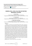
As depicted in Fig. 1, a uniform rotor of length L, diameter d, rotating at constant angular velocity
Ω, and subjected to uniform axial load P is considered. Using Timoshenko beam theory, the set of
governing equations of free vibration can be stated as (Genta, 2007)
222
222
0
y
xxx
uuu
kGA P A
zz z t
, (1-a)
222
222
0
yyy
x
uuu
kGA P A
zz z t
, (1-b)
22
22
0
yy
xx
xxpx
u
EI kGA I I
zz tt
, (1-c)
22
22
0
yy
xx
yypy
u
EI kGA I I
zz tt
, (1-d)
where ux(z,t), uy(z,t), φx(z,t) and φy(z,t) are components of displacement and rotation in x and y
directions, respectively; ρ, E and G are mass density, modulus of elasticity and shear modulus,
respectively; Also, A, Ix, Iy and Ip are cross-sectional area, moment of inertia about the x and y axis and

K. Torabi and H. Afshari
/ Engineering Solid Mechanics 4 (2016)
99
polar moment of inertia, respectively; and k is shear correction factor which depends on the shape of
the section and Poisson's ratio of material (Hutchinson, 2001).
Fig. 1. Axial-loaded Timoshenko rotor
According to Timoshenko beam theory, components of bending moment (M) and shear force (F)
in x and y directions are presented as (Genta, 2007)
yyy
xxx
xyx yy x
uu
uu
MEI MEI FkGA P FkGA P
zz zz zz
.
(2)
Using following relation for a circular section:
222
px y
IIII
.
(3)
Eqs. (1-c) and (1-d) can be written as
22
22
20
yy
xx
x
u
EI kGA I I
zz tt
.
(4-a)
22
22
20
yy
xx
y
u
EI kGA I I
zz tt
.
(4-b)
By introducing following complex variables (i
2
=-1):
xy x y
uu iu i
(5)
Eq. (1-a), Eq. (1-b), Eq. (4-a) and Eq. (4-b) reduce to
222
222
0
uuu
kGA i P A
zz z t
,
(6-a)
22
22
20
u
EI kGA i i I I
zz tt
,
(6-b)
and complex forms of bending moment and shear force (Eq. (2)) can be written as
xy xy
uu
mM iM EI f F iF kGA i P
zzz
.
(7)
Uncoupling u and φ in Eq. (6-a) and Eq. (6-b) yields the following relations:
22
22
1
Pu u
i
zkGAzkGt
.
(8-a)
x
y z
Ω
L
d
P
P

100
443
4222
224 23 2
24 32
11 21
20
P
uEPu Pu
EI I i I
kGA z kG kGA z t kGA z t
uIu Iu u
PiA
zkGt kGt t
(8-b)
Introducing ω as the circular natural frequency of whirling, ζ=z/L as the dimensionless spatial
variable and also using the method of separation of variables as
,,
it it
utLv e t e
(9)
Eq. (8-a) and Eq. (8-b) can be written in the following dimensionless form:
22 *
1is v Pv
, (10-a)
4
12
20vdvdv
, (10-b)
where the prime indicates the derivative with respect to the dimensionless spatial variable (ζ) and the
following dimensionless parameters are defined:
42
22*2
222
42 42 *
2 2
12
*
2*
21
4
221
21
21
dPAL
rs rP
Lk kGAEI
rsr
AL s P
dd
EI P
sP
(11)
In the whirling analysis of rotors, two kind of frequencies can be considered. When whirling and
spin of the rotor are in the same direction (Ωω>0), forward whirling occurs and when they are in
opposite directions (Ωω<0), backward one occurs. Solution of Eqs. (10-a) and (10-b) depends on the
sign of d2 which differs at low and high modes. In practice, lower frequencies are more important than
higher ones and d2 is a negative parameter at these modes, thus following solution can be found (Torabi
et al., 2013b):
01 1 2 2
01 1 1 1 2 2 2 2
cosh sinh cos sin
sinh cosh sin cos
vvA B C D
iv Am Bm Cm Dm
(12)
in which v0 is a complex coefficient and
222 222
22
12
12 11122112
12
ss
mm dddddd
. (13)
Also, bending moment and shear force can be written as
,,
it it
EI
mt M e f tkGAF e
L
, (14)
in which
*
1
M
FPvi
(15)
3. Basic functions
In order to derive basic functions, first, consider following definitions for trigonometric and
hyperbolic functions:
112132 42
11 1 21 1 3 2 2 4 2 2
cosh sinh cos sin
sinh cosh sin cos
SSSS
T im T im T im T im (16)
which are defined according to Eq. (12). Geometrical basic functions will be defined to satisfy
following constraints:

K. Torabi and H. Afshari / Engineering Solid Mechanics 4 (2016)
101
11
11
22
22
33
33
44
44
01 00 00 00
00 01 00 00
00 00 01 00
00 00 00 01
SS TT
SSTT
SS TT
SSTT
(17)
Now, displacement and rotation, can be stated in terms of their values at the left side of the rotor
(ζ=0) and the geometrical basic functions as:
123 4
123 4
() 0 () 0 () 0 () 0 ()
() 0 () 0 () 0 () 0 ()
vvS vS S S
vT v T T T
(18)
In order to obtain geometrical basic functions in terms of S1-T4, following relation are considered:
44
11
i
iij j ij j
jj
SASTAT
(19)
Substituting Eq. (16) and Eq. (17) into the Eq. (19), following relation will be obtained:
11
11
1111
22
22 2 222
3 333
33
33
4 444
44
44
0000 0000
0000 0000
0000
0000
0000
0000
SSTT SSTT
SSTT SSTT
ASSTT
SSTT
SSTT
SSTT
(20)
Using Eq. (20), the coefficients of Eq. (19) can be obtained as
22 11
11 22 11 22
21
21 12 21 12
21
21 12 21 12
11 22 11 22
00
00
00
00
mm
mm mm
mm
mm mm
Aii
mm mm
ii
mm mm
(21)
which leads to
122 1 11 2
11 2 2
22112
21 12
32112
21 12
412
11 2 2
1cosh cos
1sinh sin
sinh sin
cosh cos
Smm
mm
Smm
mm
i
Smm
i
Smm
12
12112
11 2 2
12
212
21 12
312 1 21 2
21 12
41122
11 2 2
sinh sin
cosh cos
1cosh cos
1sinh sin
im m
Tmm
im m
Tmm
Tmm
mm
Tmm
mm
(22)


![Hệ thống phanh Mazda CX5: [Mô tả/Đánh giá/Hướng dẫn chi tiết]](https://cdn.tailieu.vn/images/document/thumbnail/2016/20160824/khoanhi1996/135x160/6221472045851.jpg)


![Đề thi Động cơ đốt trong kết thúc học phần: Tổng hợp [năm]](https://cdn.tailieu.vn/images/document/thumbnail/2026/20260320/hoabattu2026/135x160/24841774320014.jpg)


