Chapter 21 The determination of national income
David Begg, Stanley Fischer and Rudiger Dornbusch, Economics, 6th Edition, McGraw-Hill, 2000 Power Point presentation by Peter Smith
Aggregate output in the short run
– the output the economy would produce if
n Potential output
all factors of production were fully employed n Actual output
– what is actually produced in a period – which may diverge from the potential
level
21.2
Some simplifying assumptions
n Prices and wages are fixed n The actual quantity of total output is
demand-determined – this will be a “Keynesian” model
– no government – no foreign trade
n Later chapters relax these assumptions
n For now, also assume:
21.3
Aggregate demand
n firms’ desired or planned additions to
n Given no government and no international trade, aggregate demand has two components: – Investment
n for now, assume this is autonomous
– Consumption
n households’ demand for goods and services
physical capital & inventories
n so, AD = C + I
21.4
Consumption demand
n Households allocate their income
between CONSUMPTION and SAVING
– income that households have for
n Personal Disposable Income
spending or saving
– income from their supply of factor services (plus transfers less taxes)
21.5
Consumption and income in the UK at constant 1995 prices, 1989-1998
500
i
475
450
) . n b £ (
425
l
400
e r u t i d n e p x e
375
n o p t m u s n o c d o h e s u o H
350
400
425
450
475
500
525
550
Real disposable income (£bn.)
Income is a strong influence on consumption Income is a strong influence on consumption expenditure – but not the only one. expenditure – but not the only one.
21.6
The consumption function
The consumption function shows desired aggregate The consumption function shows desired aggregate consumption at each level of aggregate income consumption at each level of aggregate income
C = 8 + 0.7 Y C = 8 + 0.7 Y
n n o o i i t t p p m m u u s s n n o o C C
With zero income, With zero income, desired consumption desired consumption is 8 (“autonomous is 8 (“autonomous consumption”). consumption”).
{{88
The The marginal propensity marginal propensity (the slope of to consume (the slope of to consume the function) is 0.7 – i.e. the function) is 0.7 – i.e. for each additional £1 of for each additional £1 of income, 70p is consumed. income, 70p is consumed.
Income Income
00
21.7
The saving function
i i
g g n n v v a a S S
The saving function shows The saving function shows desired saving at each desired saving at each income level. income level.
S = -8 + 0.3 Y S = -8 + 0.3 Y
Income Income
00
Since all income is either Since all income is either saved or spent on saved or spent on consumption, the saving consumption, the saving function can be derived function can be derived from the consumption from the consumption vice versa. function or vice versa. function or
21.8
The aggregate demand schedule
AD = C + I AD = C + I
CC
d d n n a a m m e e d d e e t t a a g g e e r r g g g g A A
II
Aggregate demand is Aggregate demand is what households plan what households plan to spend on consumption to spend on consumption and what firms plan to and what firms plan to spend on investment. spend on investment. The AD function is The AD function is the vertical addition the vertical addition of C and I. of C and I. (For now I is assumed (For now I is assumed autonomous.) autonomous.)
Income Income
21.9
Equilibrium output
i i
4545oo line line
EE ADAD
g g n n d d n n e e p p s s d d e e r r i i s s e e D D
line shows the The 45o o line shows the The 45 points at which desired points at which desired spending equals output spending equals output or income. or income. schedule, Given the ADAD schedule, Given the
equilibrium is thus at E. equilibrium is thus at E.
Output, Income Output, Income
This the point at which This the point at which planned spending equals planned spending equals actual output and income. actual output and income.
21.10
An alternative approach
I I , ,
S S
An equivalent view of An equivalent view of equilibrium is seen by equilibrium is seen by equating equating SS
planned investment (II)) planned investment (
II EE
Output, Income Output, Income
to planned saving (SS)) to planned saving (
again giving us again giving us equilibrium at E equilibrium at E
The two approaches are equivalent. The two approaches are equivalent.
21.11
Effects of a fall in aggregate demand
4545oo line line
i i
ADAD00
g g n n d d n n e e p p s s d d e e r r i i s s e e D D
ADAD11
Suppose the economy Suppose the economy starts in equilibrium starts in equilibrium at Yat Y0.0. a fall in aggregate a fall in aggregate demand to AD11 demand to AD Leads the economy Leads the economy to a new equilibrium to a new equilibrium at Yat Y11..
YY11
YY00 Output, Income Output, Income Notice that the change in equilibrium output is Notice that the change in equilibrium output is larger than the original change in AD. larger than the original change in AD.
21.12
The multiplier
n The multiplier is the ratio of the
change in equilibrium output to the change in autonomous spending that causes the change in output.
n The larger the marginal propensity to consume, the larger is the multiplier. – The higher is the marginal propensity to
save, the more of each extra unit of income “leaks” out of the circular flow.
21.13