
TNU Journal of Science and Technology
229(07): 58 - 64
http://jst.tnu.edu.vn 58 Email: jst@tnu.edu.vn
A DEEP LEARNING APPROACH FOR CREDIT SCORING
Hoang Thanh Hai1*, Than Quang Khoat2
1TNU - University of Economics and Business Administration
2Ha Noi University of Science and Technology
ARTICLE INFO
ABSTRACT
Received:
17/01/2024
Granting credit to customers is the core business of a bank. Hence,
banks need adequate models to decide to whom to approve a loan. Over
the past few years, the usage of deep learning to select appropriate
customers has attracted considerable research attention. However, the
data shortage, type of features, and data imbalance could decrease deep
learning model performance from the accuracy perspective. This study
aims to build a classifier for credit scoring based on deep learning. We
use a credit scoring dataset publicly available on the UC Irvine
Machine Learning Repository, a source of machine learning datasets
commonly used by researchers. The model architecture is designed to
be suitable for two kinds of input features, categorical and numerical
ones. Our proposed model gave a relatively high accuracy among
recent deep-learning-based models on the same dataset. We also
consider the bank profit when applying the model, which is the ultimate
goal of lenders. We found that if the banks use our model, they could
gain a significant profit.
Revised:
14/5/2024
Published:
14/5/2024
KEYWORDS
Credit Scoring
Deep Learning
Profit
Data Imbalance
Data Shortage
MỘT MÔ HÌNH HỌC SÂU CHO BÀI TOÁN XẾP HẠNG TÍN DỤNG
Hoàng Thanh Hải1*, Thân Quang Khoát2
1Trường Đại học Kinh tế và Quản trị Kinh doanh - ĐH Thái Nguyên
2Đại học Bách khoa Hà Nội
THÔNG TIN BÀI BÁO
TÓM TẮT
Ngày nhận bài:
17/01/2024
Cho vay tín dụng là hoạt động kinh doanh chủ yếu của một ngân hàng.
Do đó, các ngân hàng cần một mô hình có độ chính xác cao để quyết
định khách hàng nào được cho vay. Trong những năm gần đây, việc sử
dụng học sâu để lựa chọn khách hàng phù hợp thu hút được sự quan
tâm lớn. Tuy nhiên, việc thiếu hụt dữ liệu, sự đa dạng của loại dữ liệu,
hay mất cân bằng trong dữ liệu có thể làm giảm độ chính xác của các
mô hình phân loại dựa trên học sâu. Mục tiêu nghiên cứu của chúng tôi
trong bài báo này là xây dựng một mô hình phân loại tín dụng dựa trên
học sâu. Chúng tôi sử dụng bộ dữ liệu được công bố trên kho lưu trữ
UC Irvine Machine Learning, một kho lưu trữ các bộ dữ liệu được sử
dụng nhiều trong học máy. Kiến trúc mô hình được thiết kế để phù hợp
với hai loại dữ liệu đầu vào của mô hình, dữ liệu định tính và dữ liệu
định lượng. Mô hình được đề xuất có độ chính xác tương đối cao trong
lớp các mô hình học sâu trên cùng bộ dữ liệu. Chúng tôi cũng xem xét
lợi nhuận thu được của ngân hàng khi sử dụng mô hình. Kết quả cho
thấy mô hình mang lợi mức lợi nhuận đáng kể cho ngân hàng.
Ngày hoàn thiện:
14/5/2024
Ngày đăng:
14/5/2024
TỪ KHÓA
Xếp hạng tín dụng
Học sâu
Lợi nhuận
Mất cân bằng dữ liệu
Thiếu hụt dữ liệu
DOI: https://doi.org/10.34238/tnu-jst.9608
* Corresponding author. Email: hoangthanhhai03091988@gmail.com

TNU Journal of Science and Technology
229(07): 58 - 64
http://jst.tnu.edu.vn 59 Email: jst@tnu.edu.vn
1. Introduction
There are two main approaches to assess credit risk: the judgmental approach and the
statistical approach. A judgmental approach is a qualitative, expert-based approach whereby,
based on business experience and common sense, the credit expert will make decisions about the
credit risk [1]. The statistical one is a data-based method, where the lenders use historical data to
find the relationship between a customer’s characteristic and the binary (good or bad) target
variable. This approach has many advantages compared with the judgmental one. It is better in
terms of speed and accuracy. Moreover, it is also consistent. We no longer have to rely on the
experience, intuition, or common sense of someone.
Recently, deep learning models have been increasingly used in credit scoring, besides
classical machine learning models. This transition is partly thanks to great performances shown
by deep learning in various real-world applications like image recognition, computer vision, or
financial data analysis. However, the performance of DL-based classifiers does not really
outperform that of classifiers without deep learning techniques in several credit scoring problems.
This is partly due to the size and the type of input data. Hence, it is necessary to use suitable
methods to deal with these problems. We proposed a data augmentation technique to generate
more similar data to train model efficiently with small data. Credit data usually consist of both
numeric and categorical features, so we need to build an appropriate model architecture that can
learn two separate data types. Imbalance is also a common phenomenon with credit data, where
customers classified as Bad are normally minor. In this paper, we combined some appropriate
methods simultaneously in order to improve model performance using data encountered above
mentioned issues. We then examined model improvement by the ablation study.
Credit scoring is a binary classification problem. The lenders want to build a classifier to
divide the lenders into good and bad groups. Numerous statistical and machine learning methods
have been applied in credit scoring over the years, such as logistic regression [2], neural networks
[3], decision trees [4], or support vector machines [5]. Initially, the accuracy of these methods
appeared to be limited. Recently, the performance of machine-learning-based models has
improved considerably since the adoption of ensemble methods like bagging and boosting. Over
the last years, the application of deep learning models in credit scoring has attracted considerable
research attention. Up until now, various DL models have been applied. The most popular
models are multilayer perceptrons (MLPs), convolution neural networks (CNNs), and long short-
term memory (LSTM). LSTM networks are DL networks specifically designed for sequential
data analysis. Wang et al. [6] used an attention mechanism LSTM network to predict the
probability of user default in peer-to-peer lending. Dastile et al. [7] proposed converting tabular
datasets into images and the application of CNNs in credit scoring. Li et al. [8] constructed a two-
stage hybrid default discriminant credit scoring model based on deep forest. However, the
performance of DL-based models is not always superior to classical machine learning classifiers,
especially in case the data is small and includes various categorical features.
Making a profit is clearly the ultimate goal of any business. A credit scoring model that gives
banks no profit could not be applied in actual business activity. Therefore, considering profit
perspective when applying a classification model is crucial. Most studies consider the profit
metric as an evaluation measure for the validation process rather than as an objective to be
maximized in the training process of the model. These studies proposed some profit formula, then
assessed the bank profit of the trained model. Profit formulas vary from source to source,
depending on each author’s assumptions or each bank’s profit calculation.
The objectives of this study are twofold: (1) to conduct a classification model using a deep
learning approach that gains relatively high accuracy although the dataset is small and
imbalanced; (2) to consider the bank profit, whether it gains a profit or incurs a loss when using
the model.
TNU Journal of Science and Technology
229(07): 58 - 64
http://jst.tnu.edu.vn 60 Email: jst@tnu.edu.vn
2. Methods
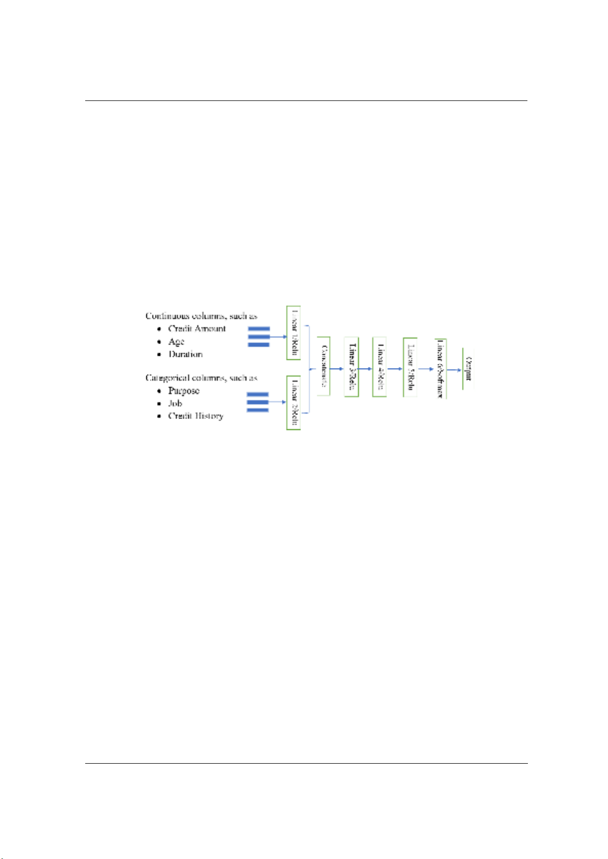
Our proposed framework consists of four stages. Firstly, we randomly split data into training
and test sets. We use the training data to train the model and the test set to evaluate the final
model. Credit datasets are often tabular data comprising various feature types, so we divide input
columns into categorical and continuous ones. The initial training set is small, so we propose a
method to augment training data. Oversampling is then applied with the training data to achieve
equal split between two target classes. Next, input columns are fed into the network through
separate layers, depending on their data category. Each type of column has its own linear layer to
learn separately before concatenating into a shared four hidden layers network. The model
architecture is shown in Figure 1. Then we train the overall network on the training set to achieve
the best model. In the third stage, the final model is evaluated using different measurements. We
do ablation study to assess the influence of each used method to the model performance. Finally,
the bank profit is considered under some assumptions. The methodology undertaken in this study
is discussed in detail in the following subsections.
Figure 1. The proposed model architecture
2.1. Data augmentation
Data augmentation is a technique of increasing the amount of data by generating new data
instances from original data. It involves making minor changes to the data or using deep learning
models to create new samples. In this study, we propose a data augmentation method by adding
noise to instances. For each original data point, we create new samples by adding a tiny change
amount to numerical features and remaining other categorical features unchanged. Let
*( ) + be the training dataset, where ( ) are the
features, is the credit status ( ) of the ith customer, ( ) are continuous
and ( ) are categorical. Set
The new continuous feature values are determined by
where is sampled from uniform distributions ( ) and is a small parameter. The
new samples corresponding to ( ) have the following form
(
)
By sampling multiple times from above uniform distributions, we have a bigger training dataset
including new sampled instances and the original ones.
2.2. Oversampling
Imbalance is common in credit scoring datasets, where the great majority of data are good
credit customers. Imbalanced data can cause deep learning models to favor the majority class
while neglecting the minority class, leading to poor performance and biased predictions [9].

TNU Journal of Science and Technology
229(07): 58 - 64
http://jst.tnu.edu.vn 61 Email: jst@tnu.edu.vn
Random oversampling involves randomly duplicating examples from the minority class and
adding them to the training class dataset. This can be repeated until the desired class distribution
is achieved in the training dataset, such as an equal split across the classes. Applying a re-
sampling strategy to obtain a more balanced dataset is considered an effective solution to the
imbalance problem [10].
2.3. Weighted cross entropy loss
Cross entropy is a commonly used loss function for classification problems. It is a measure of
how different two distributions are. In credit scoring, we are interested in the difference between
the true label and the predicted label of customers. Suppose we have a classification problem
with two classes. Let * ( ) + be the true label distribution, where each
element represents the probability of the corresponding class (( ) or ( )). Let *
( ) + be the predicted label distribution. The cross entropy between and is
given by
∑( )
The cross entropy is a non-negative value, with lower values indicating that the predicted
distribution is closer to the true distribution.
In case we want the model to pay more attention to some class than others, we use weighted
cross entropy. It is the cross entropy with each term multiplied by a weight factor. The weighted
cross entropy between and in the binary classification is
∑( )
where ( ) is the weight vector with each element represents the weight for the
corresponding class. The higher the weight, the more important the corresponding class is.
3. Experiments and Results
3.1. Data
In this study, we use German, one of the most used datasets in credit scoring literature. It is
publicly available on UC Irvine Machine Learning Repository [11]. The German dataset has 20
features of which 7 are numerical and 13 are categorical. These features include status of existing
checking account, duration in month, credit history and purpose, to mention a few. The target
variable is binary, i.e. customers are classified either as “Good” or “Bad”. The imbalance ratio is
2.33 (700 – Good, 300 – Bad). The dataset has no missing values.
3.2. Model
Table 1. Parameters and Architecture of the model
Layer
Parameters and Architecture
Input
Categorical Columns
Continuous Columns
Input shape: 13
Input shape: 7
Linear 1
in_features = 7, out_features = 100
Linear 2
in_features = 13, out_features = 100
Linear 3
in_features = 200, out_features = 200
Linear 4
in_features = 200, out_features = 100
Linear 5
in_features = 100, out_features = 50
Linear 6
in_features = 50, out_features = 2

TNU Journal of Science and Technology
229(07): 58 - 64
http://jst.tnu.edu.vn 62 Email: jst@tnu.edu.vn
The dataset was split into 70% training set and 30% test set following the common practice in
the literature [12]. We sampled four times from uniform distributions (with ) to augment
training data. The weight vector was ( ) where 10 was the weight of Good class. The new
training set has a size of 3500 (2450 – Good, 1050 – Bad) before oversampling process. The
resampled dataset has a size of 4900 (2450 – Good, 2450 – Bad), which is the final dataset fed
into the training process. Table 1 shows the parameters and architecture of the model.
The training set was used to determine the optimal weights and parameters of the best model.
The test set was used to assess the performance of the final model. The model was trained using
200 epochs and a batch size of 128. All experiments for this study were performed in Python
language using the Pytorch deep learning library. We used Adam method for optimizing
parameters.
3.3. Results
Model Performance
We assess the performance of our final model using the following metrics: Accuracy,
Precision, Recall, and Area Under Receiver Operating Characteristic Curve (AUC). All metrics
are measured after 10 random runs. Table 2 shows the model performance on the 30% test set.
The model AUC is 0.764, which is considered to be good, as it indicates that the model has good
discriminatory ability.
Table 2. Model Performance (mean standard deviation)
Accuracy
Precision
Recall
AUC
0.825 0.005
0.843 0.011
0.913 0.013
0.764 0.010
Table 3 shows the performance of our model and other related models in credit scoring for
German dataset. Although our accuracy and AUC are lower than those of some models without
deep learning techniques, they are relatively high amongst deep-learning-based classifiers.
Recently, only two deep learning techniques have been proposed for the German dataset [13].
This is likely because classifying dataset with numerous categorical features is more challenging.
With three used techniques (augmentation data, oversampling, weighted loss) and the two
separate flow architecture, our model could be a reference model for those who have similar
dataset type. Also, banks or credit institutions could consider using our model in their risk
management system.
Table 3. Performances of Related Models on German Credit Dataset
Study (Year)
Accuracy (%)
AUC
Methods
[14] (2021)
79.5
0.831
Without Deep learning techniques
[8] (2021)
81.2
0.868
Deep-learning-based
[15] (2009)
82.0
0.824
Without Deep learning techniques
[16] (2020)
84.0
0.713
Without Deep learning techniques
[17] (2018)
85.78
-----
Without Deep learning techniques
[18] (2018)
86.47
-----
Without Deep learning techniques
[7] (2021)
88.0
-----
Deep-learning-based
[19] (2020)
93.12
-----
Without Deep learning techniques
[20] (2021)
98.66
-----
Without Deep learning techniques
Ours
82.50
0.764
Deep-learning-based


![Chương trình học phần Thẩm định tín dụng [Chuẩn nhất]](https://cdn.tailieu.vn/images/document/thumbnail/2015/20150327/huynhlethingochoa/135x160/1749058_168.jpg)


![Tài liệu ôn tập môn Quản trị rủi ro ngân hàng [chuẩn nhất]](https://cdn.tailieu.vn/images/document/thumbnail/2026/20260311/hoatudang2026/135x160/60971773368958.jpg)


