
Appendix A
EQUATIONS OF MOTION
IN THE STATE
AND CONFIGURATION SPACES
A.1 EQUATIONS OF MOTION OF DISCRETE
LINEAR SYSTEMS
A.1.1 Configuration space
Consider a system with a single degree of freedom and assume that the equa-
tion expressing its dynamic equilibrium is a second order ordinary differential
equation (ODE) in the generalized coordinate x. Assume as well that the forces
entering the dynamic equilibrium equation are
•a force depending on acceleration (inertial force),
•a force depending on velocity (damping force),
•a force depending on displacement (restoring force),
•a force, usually applied from outside the system, that depends neither
on coordinate xnor on its derivatives, but is a generic function of time
(external forcing function).
If the dependence of the first three forces on acceleration, velocity and dis-
placement respectively is linear, the system is linear. Moreover, if the constants
of such a linear combination, usually referred to as mass m, damping coefficient
cand stuffiness kdo not depend on time, the system is time-invariant. The
dynamic equilibrium equation is then
m¨x+c˙x+kx =f(t).(A.1)

666 Appendix A. EQUATIONS OF MOTION
If the system has a number nof degrees of freedom, the most general form
for a linear, time invariant set of second order ordinary differential equations is
A1¨x +A2˙x +A3x=f(t),(A.2)
where:
•xis a vector of order n(nis the number of degrees of freedom of the
system) where the generalized coordinates are listed;
•A1,A2and A3are matrices, whose order is n×n; they contain the char-
acteristics (independent of time) of the system;
•fis a vector function of time containing the forcing functions acting on the
system.
Matrix A1is usually symmetrical. The other two matrices in general are
not. They can be written as the sum of a symmetrical and a skew-symmetrical
matrices
M¨x+(C+G)˙x +(K+H)x=f(t),(A.3)
where:
•M,themass matrix of the system, is a symmetrical matrix of order n×n
(coincides with A1). Usually it is not singular.
•Cis the real symmetric viscous damping matrix (the symmetric part of
A2).
•Kis the real symmetric stiffness matrix (the symmetric part of A3).
•Gis the real skew-symmetric gyroscopic matrix (the skew-symmetric part
of A2).
•His the real skew-symmetric circulatory matrix (the skew-symmetric part
of A3).
Remark A.1 Actually it is possible to write the set of linear differential Equa-
tions (A.2) in such a way that no matrix is either symmetric or skew symmetric
(it is enough to multiply one of the equations by a constant other than 1). A
better way to say this is that M,C,andKcan be reduced to symmetric matrices
by the same linear transformation that reduces Gand Hinto skew-symmetric
matrices.
Remark A.2 The same form of Equation (A.2) may result from mathematical
modeling of physical systems whose equations of motion are obtained by means of
space discretization techniques, such as the well-known finite elements method.
A.1 Equations of motion of discrete linear systems 667
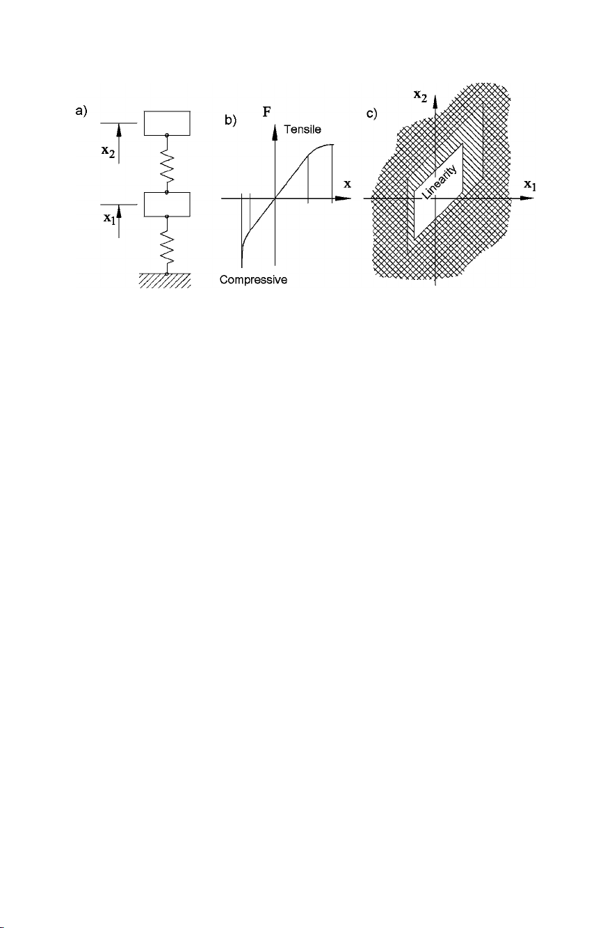
FIGURE A.1. Sketch of a system with two degrees of freedom (a) made by two masses
and two springs, whose characteristics (b) are linear only in a zone about the equilibrium
position. Three zones can be identified in the configuration space (c): in one the system
behaves linearily, in another the system is nonlinear. The latter zone is surrounded by
a ‘forbidden’ zone.
xis a vector in the sense it is a column matrix. Indeed, any set of nnumbers
may be interpreted as a vector in an n-dimensional space. This space contain-
ing vector xis usually referred to as configuration space, because any point in
this space may be associated with a configuration of the system. Actually, not
all points of the configuration space, intended to be an infinite n-dimensional
space, correspond to configurations that are physically possible for the system:
It is then possible to define a subset of possible configurations. Moreover, even
systems that are dealt with using linear equations of motion are linear only for
configurations little displaced from a reference configuration (usually the equilib-
rium configuration) and thus the linear equation (A.2) applies in an even smaller
subset of the configuration space.
A simple system with two degrees of freedom is shown in Fig. A.1a; it consists
of two masses and two springs whose behavior is linear in a zone around the
equilibrium configuration with x1=x2= 0, but behave in a nonlinear way to
fail at a certain elongation. In the configuration space, which in the case of a
system with two degrees of freedom has two dimensions and thus is a plane, there
is a linearity zone, surrounded by a zone where the system behaves in nonlinear
way. Around the latter is another zone where the system loses its structural
integrity.
A.1.2 State space
Asetofnsecond order differential equations is a set of order 2nthat can be
expressed in the form of a set of 2nfirst order equations.

668 Appendix A. EQUATIONS OF MOTION
In a way similar to above, a generic linear differential equation with constant
coefficients can be written in the form of a set of first order differential equations
A1˙x +A2x=f(t).(A.4)
In system dynamics this set of equations is usually solved in the first deriva-
tives (monic form) and the forcing function is written as the linear combination
of the minimum number of functions expressing the inputs of the system. The
independent variables are said to be state variables and the equation is written
as
˙z =Az +Bu ,(A.5)
where
•zis a vector of order m, in which the state variables are listed (mis the
number of the state variables);
•Ais a matrix of order m×m, independent of time, called the dynamic
matrix;
•uis a vector function of time, where the inputs acting on the system are
listed (if ris the number of inputs, its size is r×1);
•Bis a matrix independent of time that states how the various inputs act
in the various equations. It is called the input gain matrix and its size is
m×r.
As was seen for vector x,zis also a column matrix that may be considered
as a vector in an m-dimensional space. This space is usually referred to as the
state space, because each point of this space corresponds to a given state of the
system.
Remark A.3 The configuration space is a subspace of the space state.
If Eq. (A.5) derives from Eq. (A.2), a set of nauxiliary variables must be
introduced to transform the system from the configuration to the state space.
Although other choices are possible, the simplest choice is to use the derivatives
of the generalized coordinates (generalized velocities) as auxiliary variables. Half
of the state variables are then the generalized coordinates x, while and the other
half are the generalized velocities ˙x.
If the state variables are ordered with velocities first and then coordinates,
it follows that
z=˙x
x".
A number nof equations expressing the link between coordinates and ve-
locities must be added to the nequations (A.2). By using symbol vfor the

A.1 Equations of motion of discrete linear systems 669
generalized velocities ˙x, and solving the equations in the derivatives of the state
variables, the set of 2nequations corresponding to Eq. (A.3) is then
˙v =−M−1(C+G)v−M−1(K+H)x+M−1f(t)
˙x =v.(A.6)
Assuming that inputs ucoincide with the forcing functions f, matrices A
and Bare then linked to M,C,K,Gand Hby the following relationships
A=−M−1(C+G)−M−1(K+H)
I0
,(A.7)
B=M−1
0.(A.8)
The first nout of the m=2nequations constituting the state equation
(A.5) are the dynamic equilibrium equations. These are usually referred to as
dynamic equations. The other nexpress the relationship between the position
and the velocity variables. These are usually referred to as kinematic equations.
Often what is more interesting than the state vector zis a given linear
combination of states zand inputs u, usually referred to as the output vector.
The state equation (A.5) is then associated with an output equation
y=Cz +Du ,(A.9)
where
•yis a vector where the output variables of the system are listed (if the
number of outputs is s, its size is s×1);
•Cis a matrix of order s×m, independent of time, called the output gain
matrix;
•Dis a matrix independent of time that states how the inputs enter the
linear combination yielding the output of the system. It is called the direct
link matrix and its size is s×r. In many cases the inputs do not enter the
linear combination yielding the outputs, and Dis nil.
The four matrices A,B,Cand Dare usually referred to as the quadruple
of the dynamic system.
Summarizing, the equations that define the dynamic behavior of the system,
from input to output, are ˙z =Az +Bu
y=Cz +Du.(A.10)
Remark A.4 While the state equations are differential equations, the output
equations are algebraic. The dynamics of the system is then concentrated in the
former.
The input-output relationship described by Eq. (A.10) may be described by
the block diagram shown in Fig. A.2.


![Giáo trình Kỹ thuật chung về ô tô (Nghề: Công nghệ ô tô) - Trường Cao đẳng Bách Khoa Tây Nguyên [Mới Nhất]](https://cdn.tailieu.vn/images/document/thumbnail/2025/20251212/laphong0906/135x160/39771779074470.jpg)
![Giáo trình Kỹ thuật chung về ô tô và công nghệ sửa chữa (Nghề: Công nghệ ô tô) - Trường Cao đẳng Bách Khoa Tây Nguyên [Mới Nhất]](https://cdn.tailieu.vn/images/document/thumbnail/2025/20251212/laphong0906/135x160/23311779074471.jpg)


![Giáo trình Hệ thống nhiên liệu động cơ ô tô (CĐ) - Trường Cao đẳng Công nghiệp Thanh Hóa [Ngành Công nghệ ô tô]](https://cdn.tailieu.vn/images/document/thumbnail/2026/20260511/hoatrami2026/135x160/37511778728704.jpg)
![Giáo trình Hệ thống phanh ABS Công nghệ ô tô (CĐ) - Trường Cao đẳng Công nghiệp Thanh Hóa [Mới nhất]](https://cdn.tailieu.vn/images/document/thumbnail/2026/20260511/hoatrami2026/135x160/1901778728704.jpg)


![Giáo trình Hệ thống điện thân xe ô tô (CĐ) - Trường Cao đẳng Công nghiệp Thanh Hóa [Mới nhất]](https://cdn.tailieu.vn/images/document/thumbnail/2026/20260511/hoatrami2026/135x160/611778728708.jpg)


%20--%3e%3cdefs%3e%3cstyle%3e%20.st0%20{%20fill:%20%23fff;%20}%20.st1%20{%20fill:%20%237800fa;%20}%20%3c/style%3e%3c/defs%3e%3cpath%20class='st1'%20d='M117.78,12.18H43.11c2.9,3.47,4.65,7.94,4.65,12.82,0,5.6-2.3,10.66-6.01,14.29h76.02l7.22-13.56-7.22-13.56Z'/%3e%3cg%3e%3cpath%20class='st0'%20d='M53.58,26.17h-.59v-1.46h.59v-4.96h2.83c1.78,0,2.67.94,2.67,2.82v5.76c0,1.87-.89,2.81-2.67,2.81h-2.83v-4.96ZM55.36,21.37v3.34h1.1v1.46h-1.1v3.34h1.01c.61,0,.91-.37.91-1.1v-5.93c0-.74-.3-1.1-.91-1.1h-1.01Z'/%3e%3cpath%20class='st0'%20d='M65.99,31.14h-1.8l-.31-2.07h-2.19l-.31,2.07h-1.64l1.82-11.39h2.62l1.82,11.39ZM65.28,18.04c-.25.46-.51.77-.75.94-.21.15-.47.22-.79.22-.26,0-.57-.07-.92-.22l-.38-.15c-.14-.05-.26-.07-.37-.07-.3,0-.53.18-.71.54l-.91-.68c.25-.46.51-.77.75-.94.21-.14.48-.21.79-.21.26,0,.57.07.92.21l.38.15c.14.05.26.07.37.07.3,0,.53-.18.71-.54l.91.68ZM61.91,27.52h1.73l-.87-5.76-.87,5.76Z'/%3e%3cpath%20class='st0'%20d='M74.53,26.89v1.52c0,1.91-.89,2.86-2.67,2.86s-2.67-.95-2.67-2.86v-5.93c0-1.91.89-2.86,2.67-2.86s2.67.95,2.67,2.86v1.11h-1.69v-1.22c0-.75-.31-1.12-.93-1.12s-.93.37-.93,1.12v6.15c0,.74.31,1.11.93,1.11s.93-.37.93-1.11v-1.63h1.69Z'/%3e%3cpath%20class='st0'%20d='M81.4,31.14h-1.8l-.31-2.07h-2.19l-.31,2.07h-1.64l1.82-11.39h2.62l1.82,11.39ZM75.9,19.2l1.52-1.91h1.71l1.51,1.91h-1.61l-.76-.95-.75.95h-1.61ZM77.32,27.52h1.73l-.87-5.76-.87,5.76ZM83.1,15.99l-1.76,1.91h-1.26l1.17-1.91h1.86Z'/%3e%3cpath%20class='st0'%20d='M84.86,19.75c1.78,0,2.67.94,2.67,2.82v1.48c0,1.87-.89,2.81-2.67,2.81h-.85v4.28h-1.79v-11.39h2.64ZM84.01,21.37v3.86h.85c.58,0,.87-.36.87-1.08v-1.71c0-.71-.29-1.07-.87-1.07h-.85Z'/%3e%3cpath%20class='st0'%20d='M93.51,19.75c1.78,0,2.67.94,2.67,2.82v1.48c0,1.87-.89,2.81-2.67,2.81h-.85v4.28h-1.79v-11.39h2.64ZM92.66,21.37v3.86h.85c.58,0,.87-.36.87-1.08v-1.71c0-.71-.29-1.07-.87-1.07h-.85Z'/%3e%3cpath%20class='st0'%20d='M98.8,31.14h-1.79v-11.39h1.79v4.88h2.03v-4.88h1.83v11.39h-1.83v-4.88h-2.03v4.88Z'/%3e%3cpath%20class='st0'%20d='M105.36,24.55h2.46v1.62h-2.46v3.34h3.09v1.63h-4.88v-11.39h4.88v1.63h-3.09v3.18ZM108.17,17.29l-1.76,1.91h-1.26l1.17-1.91h1.86Z'/%3e%3cpath%20class='st0'%20d='M112.2,19.75c1.78,0,2.67.94,2.67,2.82v1.48c0,1.87-.89,2.81-2.67,2.81h-.85v4.28h-1.79v-11.39h2.64ZM111.35,21.37v3.86h.85c.58,0,.87-.36.87-1.08v-1.71c0-.71-.29-1.07-.87-1.07h-.85Z'/%3e%3c/g%3e%3ccircle%20class='st1'%20cx='25'%20cy='25'%20r='20'/%3e%3cpath%20class='st0'%20d='M32.78,19.27c2.92,0,4.43,2.55,5.28,5.33l.71,2.17c.14.38-.33.75-.71.75h-5.61c.19-.33.24-.71.09-1.08l-.75-2.45c-.43-1.32-.99-2.64-1.79-3.77.75-.57,1.65-.94,2.78-.94h0ZM25,18.38c3.25,0,4.9,2.78,5.89,5.89l.76,2.45c.14.42-.33.8-.8.8h-11.69c-.42,0-.94-.38-.8-.8l.75-2.45c.99-3.11,2.64-5.89,5.89-5.89h0ZM25,11.35c1.74,0,3.11,1.37,3.11,3.11s-1.37,3.11-3.11,3.11-3.11-1.41-3.11-3.11,1.41-3.11,3.11-3.11h0ZM17.27,19.27c1.08,0,1.98.38,2.73.94-.8,1.13-1.37,2.45-1.74,3.77l-.8,2.45c-.14.38-.05.75.09,1.08h-5.56c-.42,0-.9-.38-.75-.75l.71-2.17c.9-2.78,2.41-5.33,5.33-5.33h0ZM17.27,12.91c1.51,0,2.78,1.27,2.78,2.83s-1.27,2.83-2.78,2.83-2.83-1.27-2.83-2.83,1.27-2.83,2.83-2.83h0ZM32.78,12.91c1.56,0,2.78,1.27,2.78,2.83s-1.23,2.83-2.78,2.83-2.83-1.27-2.83-2.83,1.27-2.83,2.83-2.83h0ZM27.07,28.56v.09c0,.57-.24,1.08-.61,1.46h0v.05c-.38.33-.9.57-1.46.57s-1.08-.24-1.46-.61h0c-.38-.38-.61-.9-.61-1.46v-.09h1.41v.09c0,.19.05.38.19.47v.05c.09.09.28.19.47.19s.38-.09.47-.19v-.05c.14-.09.24-.28.24-.47t-.05-.09h1.41ZM30.99,28.56v.09c0,1.65-.66,3.16-1.74,4.24-1.08,1.08-2.59,1.79-4.24,1.79s-3.16-.71-4.24-1.79l-.05-.05c-1.04-1.08-1.7-2.55-1.7-4.2v-.09h1.41v.09c0,1.27.47,2.4,1.27,3.25h.05c.85.85,1.98,1.37,3.25,1.37s2.4-.52,3.25-1.37c.85-.8,1.37-1.98,1.37-3.25v-.09h1.37ZM34.99,28.56v.09c0,2.78-1.13,5.28-2.92,7.07-1.79,1.79-4.29,2.92-7.07,2.92s-5.23-1.13-7.07-2.92c-1.79-1.79-2.92-4.29-2.92-7.07v-.09h1.41v.09c0,2.4.94,4.53,2.5,6.08,1.56,1.56,3.72,2.5,6.08,2.5s4.52-.94,6.08-2.5c1.56-1.56,2.5-3.68,2.5-6.08v-.09h1.41Z'/%3e%3c/svg%3e)