Lesson Machine Vision: Chapter 2 - TS. Nguyen Thanh Hung

Chia sẻ: _ _ | Ngày: | Loại File: PDF | Số trang:56

Thêm vào BST

Báo xấu

2
lượt xem 1
download

Download Vui lòng tải xuống để xem tài liệu đầy đủ

Lesson "Machine Vision" Chapter 2 - Digital Image Fundamentals, compiled including the following main contents: Image Sensing and Acquisition; Image Sampling and Quantization; Some Basic Relationships Between Pixels; Basic Mathematical Tools Used in Digital Image Processing.

Chủ đề:

Bình luận(0) Đăng nhập để gửi bình luận!

Lưu

Nội dung Text: Lesson Machine Vision: Chapter 2 - TS. Nguyen Thanh Hung

TRƯỜNG ĐẠI HỌC BÁCH KHOA HÀ NỘI XỬ LÝ ẢNH TRONG CƠ ĐIỆN TỬ Machine Vision Giảng viên: TS. Nguyễn Thành Hùng Đơn vị: Bộ môn Cơ điện tử, Viện Cơ khí Hà Nội, 2021 1
Chapter 2. Digital Image Fundamentals 1. Image Sensing and Acquisition 2. Image Sampling and Quantization 3. Some Basic Relationships Between Pixels 4. Basic Mathematical Tools Used in Digital Image Processing 2
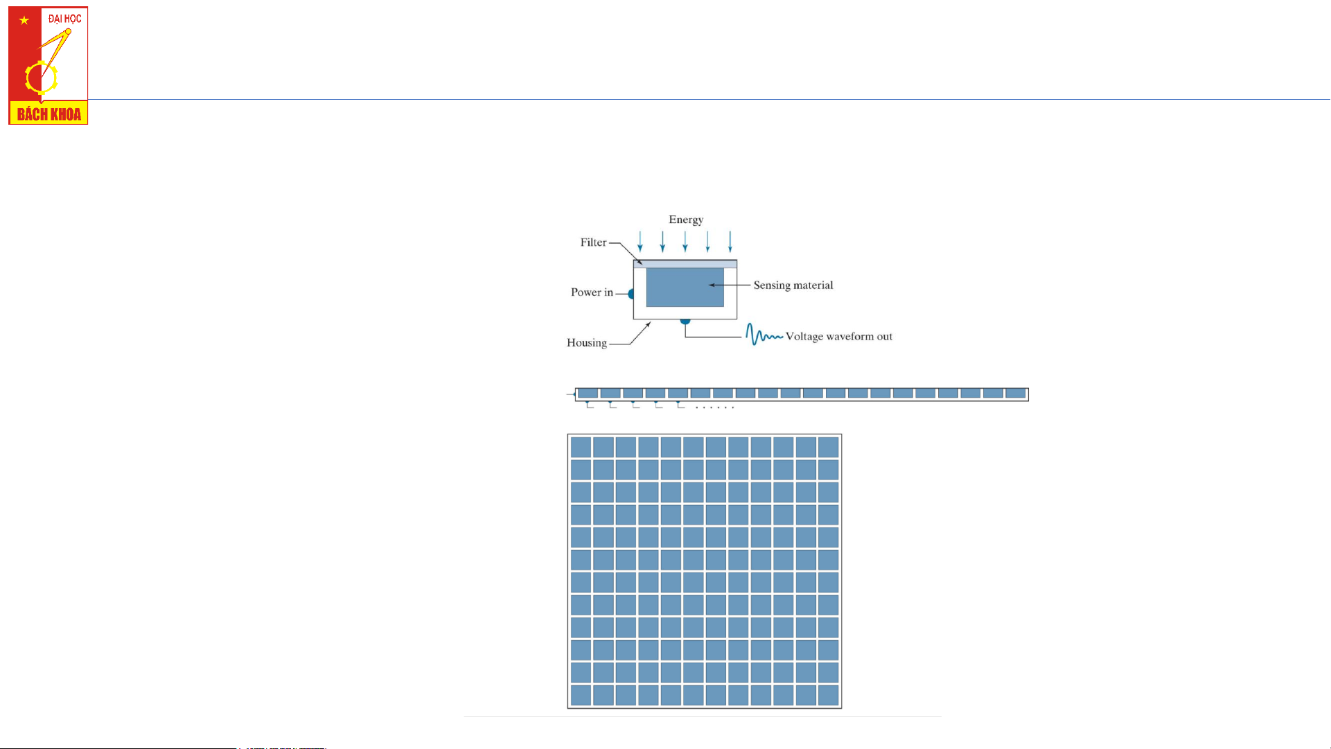
1. Image Sensing and Acquisition ❖Image Sensing and Acquisition (a) Single sensing element (b) Line sensor (c) Array sensor Rafael C. Gonzalez, Richard E. Woods, “Digital image processing,” Pearson (2018). 3
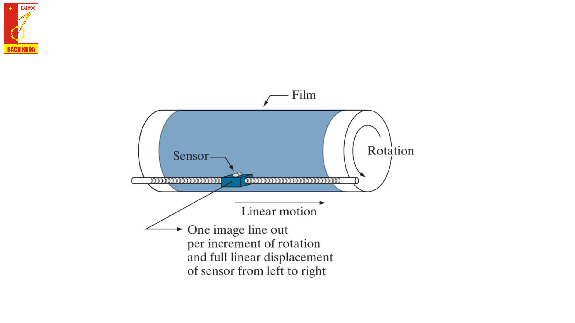
1. Image Sensing and Acquisition ❖Image Acquisition Using a Single Sensing Element Combining a single sensing element with mechanical motion to generate a 2-D image. Rafael C. Gonzalez, Richard E. Woods, “Digital image processing,” Pearson (2018). 4
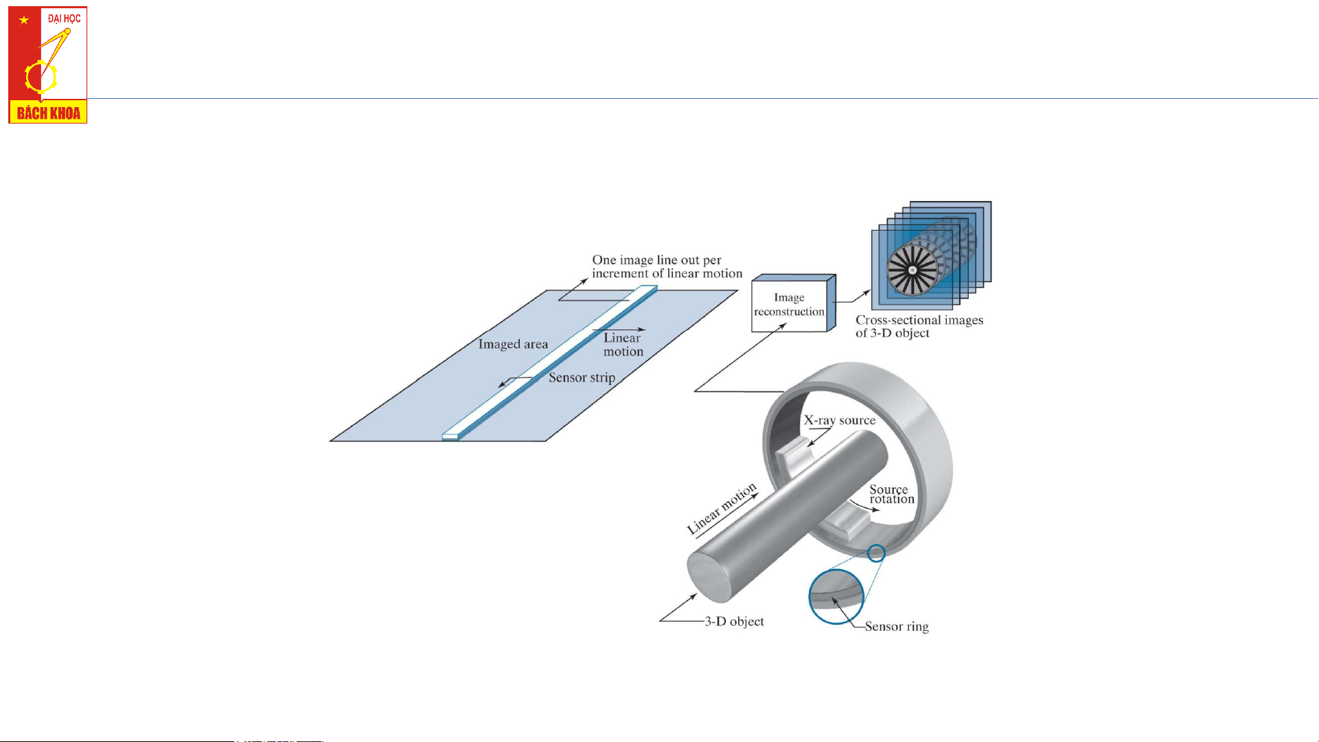
1. Image Sensing and Acquisition ❖Image Acquisition Using Sensor Strips (a) Image acquisition using a linear sensor strip (b) Image acquisition using a circular sensor strip 5 Rafael C. Gonzalez, Richard E. Woods, “Digital image processing,” Pearson (2018).
1. Image Sensing and Acquisition ❖Image Acquisition Using Sensor Arrays An example of digital image acquisition. (a) Illumination (energy) source. (b) A scene. (c) Imaging system. (d) Projection of the scene onto the image plane. (e) Digitized image. Rafael C. Gonzalez, Richard E. Woods, “Digital image processing,” Pearson (2018). 6
1. Image Sensing and Acquisition ❖A Simple Image Formation Model ➢ We denote images by two-dimensional functions of the form f(x, y) f(x, y) = i(x, y) r(x, y) • i(x, y): the amount of source illumination incident on the scene being viewed • r(x, y): the amount of illumination reflected by the objects in the scene Rafael C. Gonzalez, Richard E. Woods, “Digital image processing,” Pearson (2018). 7
Chapter 2. Digital Image Fundamentals 1. Image Sensing and Acquisition 2. Image Sampling and Quantization 3. Some Basic Relationships Between Pixels 4. Basic Mathematical Tools Used in Digital Image Processing 8
2. Image Sampling and Quantization ❖Basic Concepts in Sampling and Quantization ➢ Digitizing the coordinate values is called sampling. Digitizing the amplitude values is called quantization. (a) Continuous image. (b) A scan line showing intensity variations along line AB in the continuous image. (c) Sampling and quantization. (d) Digital scan line. (The black border in (a) is included for clarity. It is not part of the image). Rafael C. Gonzalez, Richard E. Woods, “Digital image processing,” Pearson (2018). 9
2. Image Sampling and Quantization ❖Basic Concepts in Sampling and Quantization (a) Continuous image projected (b) Result of image sampling onto a sensor array and quantization Rafael C. Gonzalez, Richard E. Woods, “Digital image processing,” Pearson (2018). 10
2. Image Sampling and Quantization ❖Representing Digital Images (a) Image plotted as a surface. (b) Image displayed as a visual intensity array. (c) Image shown as a 2-D numerical array. (The numbers 0, .5, and 1 represent black, gray, and white, respectively.) Rafael C. Gonzalez, Richard E. Woods, “Digital image processing,” Pearson (2018). 11
2. Image Sampling and Quantization ❖Representing Digital Images Coordinate convention used to represent digital images. Because coordinate values are integers, there is a one-to-one correspondence between x and y and the rows (r) and columns (c) of a matrix. Rafael C. Gonzalez, Richard E. Woods, “Digital image processing,” Pearson (2018). 12
2. Image Sampling and Quantization ❖Representing Digital Images Rafael C. Gonzalez, Richard E. Woods, “Digital image processing,” Pearson (2018). 13
2. Image Sampling and Quantization ❖Representing Digital Images ➢ The number of intensity levels: L where k is an integer. ➢ The discrete levels are equally spaced and that they are integers in the range [0, L-1] Rafael C. Gonzalez, Richard E. Woods, “Digital image processing,” Pearson (2018). 14
2. Image Sampling and Quantization ❖Representing Digital Images ➢ The number, b, of bits required to store a digital image is ➢ When M = N: Number of megabytes required to store images for various values of N and k Rafael C. Gonzalez, Richard E. Woods, “Digital image processing,” Pearson (2018). 15
2. Image Sampling and Quantization ❖Linear vs. Coordinate Indexing ➢ coordinate indexing or subscript indexing (x, y) vs linear indexing () Illustration of column scanning for generating linear indices. Shown are several 2-D coordinates (in parentheses) and their corresponding linear indices. Rafael C. Gonzalez, Richard E. Woods, “Digital image processing,” Pearson (2018). 16
2. Image Sampling and Quantization ❖Spatial and Intensity Resolution ➢ Spatial resolution is a measure of the smallest discernible detail in an image. ➢ Dots per unit distance is a measure of image resolution used in the printing and publishing industry. In the U.S., this measure usually is expressed as dots per inch (dpi). ➢ Intensity resolution is the number of bits used to quantize intensity. Effects of reducing spatial resolution. The images shown are at: (a) 930 dpi, (b) 300 dpi, (c) 150 dpi, and (d) 72 dpi. Rafael C. Gonzalez, Richard E. Woods, “Digital image processing,” Pearson (2018). 17
2. Image Sampling and Quantization ❖Spatial and Intensity Resolution (a) 256-level image. (b)-(d) Image displayed in 128, 64, and 32 intensity levels, while keeping the image size constant. (e)-(h) Image displayed in 16, 8, 4, and 2 intensity levels. Rafael C. Gonzalez, Richard E. Woods, “Digital image processing,” Pearson (2018). 18
2. Image Sampling and Quantization ❖Spatial and Intensity Resolution (a) Image with a low level of detail. (b) Image with a medium level of detail. (c) Image with a relatively large amount of detail. Rafael C. Gonzalez, Richard E. Woods, “Digital image processing,” Pearson (2018). 19
2. Image Sampling and Quantization ❖Spatial and Intensity Resolution ➢ Observe that isopreference curves tend to become more vertical as the detail in the image increases. Representative isopreference ➢ This result suggests that for images with curves for the a large amount of detail only a few three types of images intensity levels may be needed. Rafael C. Gonzalez, Richard E. Woods, “Digital image processing,” Pearson (2018). 20