90 Journal of Mining and Earth Sciences Vol. 65, Issue 6 (2024) 90 - 98
The initial research results on the improvement of
offshore axial pile capacity calculation using CPTu
data at block A, offshore Vietnam
Can Thanh Truong1,*, Long Kim Le2, Quyen Van Le3
1 Seahorse Marine & Energy JSC, Ba Ria – Vung Tau, Vietnam
2 PTSC Geos & Subsea Services Co, Ba Ria – Vung Tau, Vietnam
3 Freelance Consultant in Geotechnical Research, Hanoi, Vietnam
ARTICLE INFO
ABSTRACT
Article history:
Received 28th July 2024
Revised 27th Oct. 2024
Accepted 6th Nov. 2024
This paper presents the use of CPTu data in calculation of offshore axial
pile capacity based on the CPT-based methods recommended in Appendix
C of API RP 2GEO (2014) which are the Simplified ICP-05 Method (Method
1); Offshore UWA-05 Method (Method 2); Fugro-05 Method (Method 3);
and NGI-05 Method (Method 4). Formerly, the strength values of
cohesionless layers were usually taken from onshore laboratory results or
if there were none done, the values were generally assumed based on
recommendations of API RP 2A-WSD (2000) standard which often
resulted in unconservative axial pile capacity. With the availability of
CPTu data which better reflects the in-situ soil conditions, the selection of
design parameters for cohesionless layers is improved and consequently,
the improved axial capacity calculation both in tension and compression.
The improvement in predicted axial pile capacity allows better pile design
(for example, choice of pile length, optimization of pile diameter) and
hence the economical aspects of the final design at a later design stage.
Results from the analyses by CPT-based methods indicate that Method 1,
2 and 3 produce comparable results of capacities in both compression and
tension, whereas Method 4 shows somewhat a deviation from the other 3
methods. Hence, a conservative approach to using the capacities
calculated by method 4 and especially the API RP 2A-WSD (2000) method
should be exercised properly by applying appropriate safety factors.
Copyright © 2024 Hanoi University of Mining and Geology. All rights reserved.
Keywords:
API RP 2A-WSD,
API RP 2GEO,
Axial pile capacity,
Calculation and prediction,
CPTu,
CPT-based methods,
The offshore.
_____________________
*Corresponding author
E - mail: candytruong@searhorse.com.vn
DOI: 10.46326/JMES.2024.65(6).09

Can Thanh Truong et al./Journal of Mining and Earth Sciences 65(6), 90 - 98 91
1. Introduction
The prediction of axial pile capacity is a
critical component in offshore foundation design,
particularly for structures such as wind turbines,
oil platforms, and other marine infrastructure.
Offshore soil conditions can vary significantly due
to the complex interaction of geological history,
climate change, and human activities, making
accurate prediction methods essential for both
design and economic efficiency. Traditionally,
methods such as the API RP 2A-WSD (2000) have
been used to estimate axial capacity. However,
many studies have shown that these methods
often overestimate capacities, leading to
unconservative pile designs (Kolk & Der Velde,
1996). These discrepancies have driven the
adoption of more advanced, data-driven methods.
In recent years, the use of the Cone
Penetration Test with pore pressure
measurements (CPTu) has gained prominence,
providing better in-situ soil characterization,
especially for cohesionless soils, than older
laboratory-based methods. Studies by Mayne
(2007) have demonstrated that CPT data offers
more accurate predictions of pile behavior under
both tensile and compressive loads, resulting in
improved design parameters for axial pile
capacity calculations. CPT-based methods such as
those recommended by API RP 2GEO (2014) have
been widely accepted in the offshore engineering
community. These methods provide more
accurate capacity estimates, reducing the need for
conservative safety factors, as they are based on
direct correlations of soil resistance with CPT
measurements.
Recent advancements in machine learning
have also contributed to improving pile capacity
predictions. Nguyen et al. (2024) demonstrated
that machine learning techniques could be used to
enhance the prediction of base resistance in long
piles, particularly in soft soils, by leveraging
extensive datasets from field tests. Their study
shows how settlement influences the base
resistance of long piles and provides more
accurate assessments of pile behavior compared
to conventional empirical methods. This study
applies CPT-based methods to Block A offshore
Vietnam, integrating data from both boreholes
and CPTu measurements to derive more accurate
design parameters. By leveraging these advanced
methods, the study aims to improve the
prediction of axial pile capacity for offshore
structures, offering potential optimizations in
terms of pile length and diameter, thus reducing
construction costs without compromising safety.
2. Project description and theory of pile
capacity’s calculation method
2.1. Background information
In 2014, a geotechnical site investigation was
performed to extract soil conditions for the
development of the proposed ST-PIP (Song Tinh -
Production Injection Platform) and ST-LQ (Song
Tinh - Living Quarter) platforms. The fieldwork at
the location comprised one 140.0-m Sample
borehole and one 140.0-m CPT hole, designated
as ST-LQ and ST-PIP respectively. These
boreholes are about 148 m apart. The data
obtained from both holes are combined in order
to generate hypothetical soil parameters for the
purpose of pile foundation design. The
hypothetically combined location would be
referred to as ST-LQ/PIP Location. The
engineering analyses are for 60-in. dia. pipe piles.
The water depth of the final investigated
locations is extracted from the survey and
presented in Table 1 below.
2.2. Soil properties and stratigraphy
The soil conditions as revealed at the ST-
PIP/LQ Location indicate that they consist of
alternating granular and cohesive materials from
mudline to the final investigated depth of 140 m.
All the soil samples collected offshore were
transferred to an onshore laboratory for testing
soil properties such as grain size analyses,
Atterberg limit analyses, undrained
unconsolidated triaxial tests, consolidation tests,
Table 1. Water depths of referenced locations.
Borehole
Designation
Observed
Water Depth
[m]
Final
Investigated /Pile
Driven Depth [m]
BH ST-LQ
(Sample)
55.0
140
CPTU ST-
PIP
55.2
140

92 Can Thanh Truong et al./Journal of Mining and Earth Sciences 65(6), 90 - 98
carbonate content tests and consolidated drained
triaxial tests.
From the results of onshore laboratory tests,
the clays are generally of low plasticity with
Liquid Limits (wL’s) of 23 to 46% and stiff to very
stiff in consistency.
The sand/silty sand layers are generally
inferred to be medium dense to dense in relative
density based on CPT data at various depths.
Silt/silt with sand/sandy silt layers are
encountered from about 40.6 to 43.6 m, 56.8 to
64.0 m and 90 to 93.6 m. Coralline gravel and
siliceous carbonate sand layers are observed from
about 9.6 to 13.4 m and 13.4 to 15.2 m
respectively with carbonate content ranging
between 71% and 93%. A silty gravel with sand
layer is present from 37.6 to 40.6 m.
The strength data together with all the other
available laboratory classification test data are
used to determine the hypothetical soil
stratigraphy. The hypothetical stratigraphy at the
location is presented in Table 2.
2.3. Interpretation of piezocone penetration test
(CPTu) data
Cone penetrometer test results were used to:
▪ Interpret material properties;
▪ Determine stratigraphy and soil
conditions;
▪ Select appropriate parameters for
granular soils and inferred undrained
shear strength for clays.
The cone resistance and pore pressure data
obtained during this study were used to interpret
undrained shear strength of cohesive soils and to
estimate the relative densities of granular soils.
Sleeve friction data, also presented as friction
ratio (defined as the ratio of sleeve friction to
point resistance expressed as a percent), as well
as the measured excess pore pressure, were used
to assess soil characteristics.
2.3.1. Data for interpretation of CPTu data
The ratio of sleeve to cone tip resistance and
the excess pore pressure readings generally
supports the clay and sand/silt classification, and
readily identifies the stratified layers of sand and
silt soils.
2.3.2. Estimate of shear strength in cohesive soils
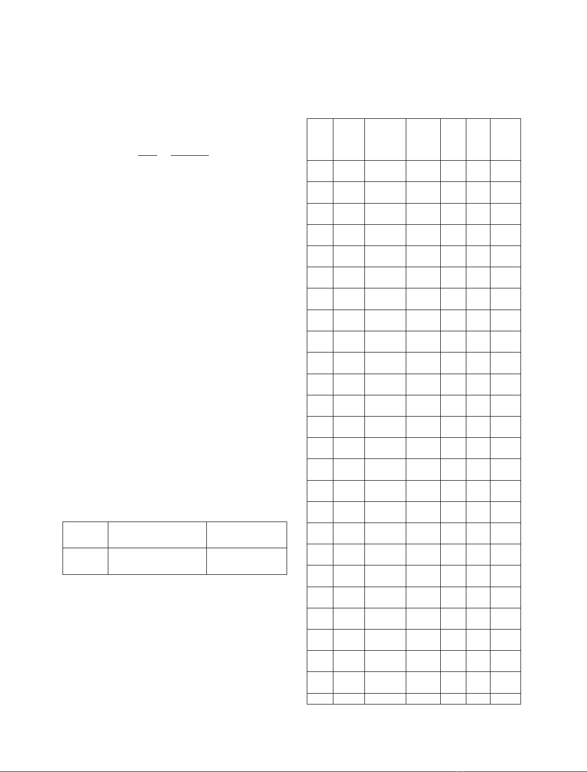
Table 2. Hypothetical Soil Stratigraphy – ST-LQ/PIP
Location (Field report at Block A, offshore Vietnam).
No.
Depth (m)
Inferred Description
1
0÷1.6
Loose silty fine SAND
2
1.6÷3.7
Medium dense to dense
silty fine SAND
3
3.7÷6
Very dense silty fine SAND
4
6÷7
Medium dense silty fine
SAND
5
7÷7.6
Stiff lean CLAY
6
7.6÷9.6
Medium dense to dense
silty fine SAND
7
9.6÷13.4
Silty CORRALLINE GRAVEL
with sand
8
13.4÷15.2
Silty siliceous carbonate
fine SAND
9
15.2÷24
Stiff to very stiff lean CLAY
10
24÷28.4
Medium dense silty fine
SAND
11
28.4÷37.6
Very stiff to hard lean CLAY
12
37.6÷40.6
Medium dense silty
GRAVEL with sand
13
40.6÷43.6
SILT with sand
14
43.6÷47.5
Medium dense to dense fine
SAND
15
47.5÷50.8
Very stiff CLAY
16
50.8÷56.8
Very stiff to hard lean CLAY
17
56.8÷64
Sandy SILT
18
64÷73.8
Stratified silty fine SAND
and very stiff CLAY
19
73.8÷90
Very stiff lean CLAY
20
90÷93.6
SILT with sand
21
93.6÷99
Very stiff lean CLAY
22
99÷120.4
Dense silty fine to medium
SAND
23
120.4÷122
Stratified very stiff lean
CLAY and silty SAND
24
122÷125
Medium dense to dense
silty fine to medium SAND
25
125÷130
Hard lean CLAY
26
130÷133
Medium dense calcareous
silty fine SAND
27
133÷135.5
Very stiff CLAY
28
135.5÷138.2
Medium dense silty fine
SAND
29
138.2÷140
Stratified silty fine SAND
and very stiff to hard CLAY
Can Thanh Truong et al./Journal of Mining and Earth Sciences 65(6), 90 - 98 93
Cone penetrometer results can be used to
estimate shear strength for cohesive materials.
CPTu results were correlated with the undrained
shear strength measured in laboratory tests using
the equation given as follows Schmertmann
(1975):
𝑐𝑢=𝑞𝑛𝑒𝑡
𝑁𝑘𝑡 =𝑞𝑡−𝜎𝑣𝑜
𝑁𝑘𝑡
(1)
Where: cu - undrained shear strength; qt -
corrected CPTu tip resistance; qnet - net cone
resistance; σvo - total overburden pressure,
(including hydrostatic); and Nkt = cone factor.
As discussed by Schmertmann (1975), the
value of Nkt depends on many variables such as:
▪ Method of determining the reference
undrained shear strength;
▪ In-situ soil stress condition;
▪ Stress history;
▪ Soil structure;
▪ Sensitivity;
▪ Plasticity characteristics;
▪ Type of penetrometer cone;
▪ Mode of CPTu operation and rate of
penetration.
The Nkt values of 15 and 20 are recommended
to be used to a depth of 24 m. For the cohesive
materials below 24 m, the Nkt values adopted are
20 and 25.
3. Axial pile capacity calculation
3.1. Analysis method for axial pile capacity
Table 3 summarizes the analysis methods for
axial pile capacity used in this article.
Table 3. Analysis methods for axial pile capacity.
Method
Cohesive Soil
Model
Frictional
Model
-
Kolk & Van der
Velde (1996)
CPT-based
Methods*
* CPT-based Methods are based on the
Simplified ICP-05, Offshore UWA-05, Fugro-05
and NGI-05 methods as per API RP 2GEO (2014)
Annex C. The hypothetical design soil parameters
are tabulated in Table 4.
3.2. Ultimate axial pile capacity of driven piles
Analyses of axial pile capacity were
performed using the procedures described in the
Kolk & Der Velde (1996) Method for the cohesive
layers.
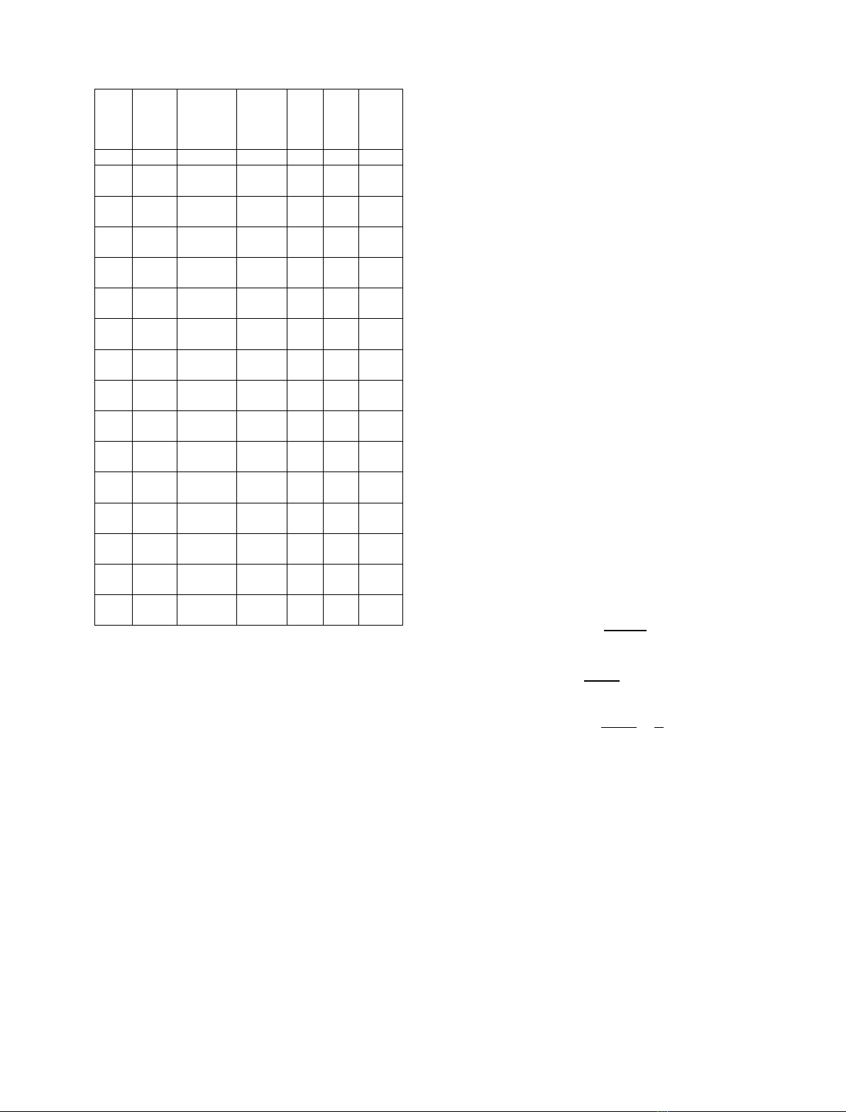
Table 4. Parameters for axial pile capacity model –
CPT-based methods.
Depth
from
to
[m]
Ground
unit
name
Ground
unit
behaviour
UW
[kN/m3]
qc
[MPa]
cu
[kPa]
Delta
[deg]
0.0
1.6
Sand
Frictional
20.3
20.3
0.8
1.2
-
27.0
1.6
3.7
Sand
Frictional
20.5
20.5
4.0
4.0
-
28.8
3.7
6.0
Sand
Frictional
19.5
19.5
12.0
12.0
-
28.8
6.0
7.0
Sand
Frictional
19.2
19.2
4.0
4.0
-
28.8
7.0
7.6
Clay
Cohesive
19.4
19.4
-
50.0
50.0
-
7.6
8.3
Sand
Frictional
19.7
19.7
18.0
18.0
-
28.8
8.3
9.6
Sand
Frictional
19.7
19.7
10.5
10.5
-
28.8
9.6
13.4
Coral
Frictional
8.8
18.8
6.0
6.0
-
23.3
13.4
15.2
Sand
Frictional
19.1
19.1
4.0
4.0
-
28.8
15.2
17.3
Clay
Cohesive
19.3
19.3
-
120.0
80.0
-
17.3
20.0
Clay
Cohesive
19.3
19.3
-
80.0
120.0
-
20.0
22.8
Clay
Cohesive
19.3
19.3
-
120.0
50.0
-
22.8
24.0
Clay
Cohesive
19.3
19.3
-
50.0
140.0
-
24.0
28.4
Sand
Frictional
21.0
21.0
8.0
8.0
-
28.8
28.4
34.2
Clay
Cohesive
20.0
20.0
-
110.0
110.0
-
34.2
37.6
Clay
Cohesive
20.0
20.0
-
110.0
200.0
-
37.6
40.6
Gravel
Frictional
19.9
19.9
8.0
8.0
-
22.8
40.6
43.6
Silt
Frictional
20.2
20.2
5.5
5.5
-
28.8
43.6
47.5
Sand
Frictional
20.0
20.0
13.0
13.0
-
28.8
47.5
50.8
Clay
Cohesive
19.4
19.4
-
105.0
105.0
-
50.8
56.8
Clay
Cohesive
20.0
20.0
-
120.0
170.0
-
56.8
64.0
Silt
Frictional
20.4
20.4
12.0
12.0
-
28.8
64.0
73.8
Sand
Frictional
19.9
19.9
6.0
6.0
-
28.8
73.8
90.0
Clay
Cohesive
19.7
19.7
-
125.0
125.0
-
90.0
93.6
Silt
Frictional
19.0
19.0
10.0
10.0
-
28.8
93.6
Clay
Cohesive
19.8
-
130.0
-
94 Can Thanh Truong et al./Journal of Mining and Earth Sciences 65(6), 90 - 98
Depth
from
to
[m]
Ground
unit
name
Ground
unit
behaviour
UW
[kN/m3]
qc
[MPa]
cu
[kPa]
Delta
[deg]
96.8
19.8
130.0
96.8
99.0
Clay
Cohesive
19.8
19.8
-
130.0
170.0
-
99.0
101.7
Sand
Frictional
20.1
20.1
37.0
37.0
-
25.6
101.7
103.5
Sand
Frictional
20.1
20.1
12.0
12.0
-
25.6
103.5
105.3
Sand
Frictional
20.1
20.1
37.0
37.0
-
25.6
105.3
120.4
Sand
Frictional
20.1
20.1
42.0
42.0
-
25.6
120.4
122.0
Sand
Frictional
20.0
20.0
14.0
14.0
-
26.6
122.0
123.0
Sand
Frictional
20.8
20.8
30.0
30.0
-
26.6
123.0
125.0
Sand
Frictional
20.8
20.8
36.0
36.0
-
26.6
125.0
127.4
Clay
Cohesive
19.6
19.6
-
200.0
200.0
-
127.4
130.0
Clay
Cohesive
19.6
19.6
-
200.0
240.0
-
130.0
133.0
Sand
Frictional
20.7
20.7
21.0
21.0
-
28.8
133.0
135.5
Clay
Cohesive
20.5
20.5
-
150.0
150.0
-
135.5
137.0
Sand
Frictional
20.4
20.4
11.0
11.0
-
28.8
137.0
138.2
Sand
Frictional
20.4
20.4
26.0
26.0
-
28.8
138.2
140.0
Sand
Frictional
19.8
19.8
8.0
8.0
-
28.8
The CPT-based Methods are used to compute
axial capacities in the frictional layers.
The four recommended CPT-based methods
in API RP 2GEO (2014) Annex C are listed as
follows:
▪ Simplified ICP-05 Method (Method 1);
▪ Offshore UWA-05 Method (Method 2);
▪ Fugro-05 Method (Method 3);
▪ NGI-05 Method (Method 4).
Ultimate axial pile capacity curves of the
proposed 60-in. dia. pipe pile under compression
and tensile loading generated are presented in
Figures 2 and 3.
As per the Client’s instruction, the target
depths 60-in. dia. pile are 110 m. The pile weight
has not been taken into account in pile capacity
curves.
Friction and end-bearing contributions to
pile capacity are assumed to be uncoupled. Hence,
for all methods, the ultimate axial pile capacity in
compression, Qc, and in tension, Qt, of plugged
open-ended piles is determined by Equations (2)
and (3).
𝑄𝑐=𝑄𝑓,𝑐 +𝑄𝑝=𝜋𝐷∫𝑓𝑐(𝑧)𝑑𝑧+𝑞𝐴𝑝
(2)
𝑄𝑡=𝑄𝑓,𝑡 =𝜋𝐷∫𝑓𝑡(𝑧)𝑑𝑧
(3)
Where: Qc - the axial pile ultimate capacity in
compression, in force units; Qt - the axial pile
ultimate capacity in tension, in force units; Qf,c - the
shaft friction capacity in compression, in force
units; Qf,t - the shaft friction capacity in tension, in
force units; Qp - the end bearing capacity, in force
units; fc(z) - the unit shaft friction in compression,
in stress units, which is a function of depth,
geometry and soil conditions; ft(z) - the unit shaft
friction in tension, in stress units, which is a
function of depth, geometry and soil conditions; z
- the depth below the original seafloor; q - the unit
end bearing at the pile tip, in stress units; D - the
pile outside diameter; Ap - the gross end area of
the pile, Ap = πD2/4 .
The unit shaft friction formulae for open-
ended steel pipe piles for CPT-based methods 1, 2,
and 3 can all be considered as special cases of the
general formula:
𝑓(𝑧)=𝑢𝑞𝑐(𝑧)(𝑝′𝑜(𝑧)
𝑝𝑎)𝑎
×𝐴𝑟𝑏⌊𝑚𝑎𝑥(𝐿−𝑧
𝐷,𝑣)⌋−𝑐
× [𝑡𝑎𝑛𝛿𝑣]𝑑× [𝑚𝑖𝑛(𝐿−𝑧
𝐷×1
𝑣,1)]𝑒
(4)
Where: f(z) - the unit shaft friction, in stress
units, which is a function of depth, geometry and
soil conditions; qc(z) - the CPT cone-tip resistance
at depth, z, in stress units; p’o(z) - the effective
vertical stress at depth z; pa - the atmospheric
pressure, in stress units, (e.g. pa = 100 kPa); Ar - the
pile displacement ratio; L - the embedded length
of the pile below the original seafloor; δcv - the
sand constant volume friction angle at the
interface between the sand and the pile wall.
The values of a, b, c, d, e, u and v are unit shaft
friction parameter values for driven open-ended
steel piles as described in API RP 2GEO (2014)
Annex C.


![Tài liệu giảng dạy Vi tích phân A2 [chuẩn nhất]](https://cdn.tailieu.vn/images/document/thumbnail/2026/20260323/hoatudang2026/135x160/54651774420904.jpg)


![Tài liệu giảng dạy Hình học Affine và Euclide [chuẩn nhất]](https://cdn.tailieu.vn/images/document/thumbnail/2026/20260323/hoatudang2026/135x160/52531774414221.jpg)


