
* Corresponding author.
E-mail address: hoilq@neu.edu.vn (Q. H. Le)
© 2019 by the authors; licensee Growing Science, Canada.
doi: 10.5267/j.dsl.2019.3.002
Decision Science Letters 8 (2019) 225–232
Contents lists available at GrowingScience
Decision Science Letters
homepage: www.GrowingScience.com/dsl
Ownership, technology gap and technical efficiency of small and medium manufacturing firms
in Vietnam: A stochastic meta frontier approach
Thi Minh Nguyena, Quoc Hoi Lea*, Thi Van Hoa Trana, and Minh Ngoc Nguyena
aNational Economics University, Vietnam
C H R O N I C L E A B S T R A C T
Article history:
Received February 7, 2019
Received in revised format:
March 10, 2019
Accepted March 16, 2019
Available online
March 16, 2019
The ownership - efficiency relationship in a firm has always been an important topic. In this
paper, we focus on the state owned versus non-state-owned status of Vietnamese manufacturing
firms, to shed light into the relationship between these two variables when using a more state-
of-the-art method as a stochastic meta-frontier method. Applying the method for two periods:
one during the global economic crisis and the other after the end of the crisis, the study
determines that in both periods, there was a strong evidence that non-state-owned firms
performed much better than state owned counterpart. We also found that the difference became
even larger during the harsh time and sub-industries with non-state-owned firms could
outperform the state-owned firms, significantly.
.2018 by the authors; licensee Growing Science, Canada©
Keywords:
Ownership
Technology gap
Technical efficiency
Small and medium manufacturing
firms
Vietnam
1. Introduction
Vietnam is on the way towards to a more market-oriented economy. From the legal perspective, the
Enterprise Law 2005 and more recently the Enterprise Law 2014 help to reduce the difference in the
ways state owned enterprises (SOE) and non-SOE are treated by law. From the practical perspective,
more enterprises have been privatized and that makes the private sector become more important part of
the economy. However, the difference still exists, in which SOE are regarded as less efficient despite
the fact that they get more preferential treatments compared with their non-SOE counterparts.
With the growing role of the private sector in the economy, a question remains is how the non-SOE
firms perform compared with the SOE counterparts. On one hand, non-SOE firms do not have serious
conflict of interest as in SOE firms, people who control the right of the firms may have not cash flow
right at all. As such, non-SOE firms may be more flexible and have more incentive to take risk than
SOE firms. Therefore, we may expect that the variation in firms’ performance among non-SOE firms
would be higher than that among SOE firms. As such, we would observe a technology gap between the
production frontiers of the two groups, and the difference in efficiency as well. As technical efficiency

226
is an important determinant of a firm’s competitiveness, studies about firms’ technical efficiency are
rich and still growing. The studies often use different approaches, either parametric, non-parametric, or
semi-parametric approaches. The non-parametric approaches are originally based on the Data
Envelopment Analysis (DEA) method proposed by Charnes et al. (1978) from the idea of Farrell
(1957). This method was used extensively in studies about firm’s technical efficiency. However, when
applied to different sets of data - the same industry for different economies or different sub industries
in the same economy – the use of DEA to estimate firms’ technical efficiency could be unjustified. As
different sets of firms may use different sets of technology (Hayami, 1969) which cannot be described
by the same set of parameters of the problem. In addition, the meta-DEA method proposed by Battese
et al. (2004) and O’Donnell et al. (2008) has been extensively used to solve for efficiency measurement.
Since then, the method has been applied in various studies (e.g. Goyal et al., 2018; Hafezalkotob et al.,
2015; Naceur et al., 2011).
Another line of studies is to use the parametric approaches, which are originally based on stochastic
frontier analysis (SPA), proposed simultaneously by Aigner et al. (1977) and Meeusen and Van den
Broeck (1977). The idea of the SFA is that, firms are no longer assumed to be at their most efficient,
hence the inefficient component should be added in the production function. The inefficient component
of a firm is measured as the distance between the firm output and the output of the most efficient firm
using the same bundle of input (for the SFA with the production function, and the same idea for the
SFA with the cost function). Wang and Wong (2016), for example, used SFA to study the technical
efficiency of Chinese manufacturing firms. Using a set of 12000 firms, they found that foreign direct
investment (FDI) would not create the horizontal effect, i.e. the presence of FDI firms would not
improve technical efficiency of the firms in the same industry. They also found that FDI had a mixed
vertical effect and could improve the technical efficiency for the firms in upstream industries but not
for the firms in downstream industries.
In Vietnam, there have been also many studies about technical efficiency, (see Ho, 2016; Nguyen;
2005, for example). These studies used normal DEA and SFA methods, hence may suffer from the
mentioned above problem. Our study differs the previous works: first, we use the state-of-art method
and focus on ownership in particular; secondly, we compare the situation in the time of economic crisis
(2011) and when the crisis was over (2016). As such, we hope that the paper can bring about some
insight into the existing literature. The structure of the paper is as followed: the following section will
briefly introduce the methodology, the next section presents our model and estimated result, and the
last section presents the conclusion to summarize the contribution of the paper.
2. Methodology
This section briefly presents the method used in this study, which is Stochastic Meta - frontier- analysis.
We start by introducing the SFA approach and then move to the Stochastic Meta Frontier analysis.
2.1 The SFA approach
In the SFA approach, the production function of a firm can be expressed as (Aigner et al, 1977):
f(x, ). .e
uv
ye
(1)
where y represents the output, x denotes the vector of inputs,
is associated with the vector of
parameters to be estimated; v is the normal random error, which is assumed to be independent,
identically distributed, and u reflects the firm’s inefficiency. In the setup, u is assumed to be
independent from v and u is non-positive and follows some specific distribution. It can be seen from
Eq. (1) that if all firms are efficient then 0u
. So normal practice of estimating the input shares is a
special case of Eq. (1) when assuming that the production is efficient. Technical efficiency of firm i
can be calculated as:
.
(,)
i
u
i
iv
i
y
TE e
fx e

T. M. Nguyen et al. / Decision Science Letters 8 (2019)
227
The TE of firm i lets us know how much output of the firm could be produced using the same amount
of inputs when the firm works, efficiently. In practice, the function f(.) can take a common Cobb-
Douglas form, and Eq. (1) can be expressed as:
01 1
ln(y) ln( ) .. ln( )
kk
x
xvu
or translog form as:
01 1
ln(y) ln( ) .. ln( ) ln( ) ln( )
kk i j
ij
x
xxxvu
The model can be estimated using maximum likelihood (ML) method with v following a Normal, and
u follow either half-normal, exponential, or truncated normal distribution.
2.2 Meta – SFA approach
The above method is appropriate if all firms choose the same technology. However, in practice, firms
may choose different technologies, depending on resource endowment, for instance. Hence if the firms
in study are clustery heterogenous in their chosen technology, the meta production approach would be
more appropriate. In that case, the production function of firm i in group j can be stated as follows,
,,
f(x, ). .e
ij ij
uv
jj j
ii
ye
. (2)
Hence the technical efficiency for firm i in group j is as follows,
,ij
u
j
i
TE e.
The meta frontier production function for all M groups is also expressed as follows,
(, ) (, )
T
ij
u
jj j Tj j
ii
f
xfxe
. (3)
In (.)
T
f is the production frontier for all groups, ,
T
ij
U indicates the difference in the frontier of each
group to the frontier of all groups. Hence the ratio ,
,
,
()
e
()
M
ij
j
u
ij
T
ij
fx
fx
measures the technology gap ratio
,ij
TGR between the technology of the firm i in group j and the best technology for all groups. The meta-
technical efficiency, measures the distance between the actual output of firm i group j and the meta-
frontier production function, MTEij can be written as:
,, ,ij ij ij
M
TE TE xTGR. (4)
The estimation
Huang et al. (2014) proposed a method to estimate meta-technical efficiency MTE and technical gap
ratio (TGR) as followed:
The first step: This step will use the mentioned above SFA method to estimate the frontier for each
group to get ,
ˆ()
jij
f
x using Eq. (2). This step will also produce technical efficiency for each firm,
j
i
TE
Second step: In this step, the estimated group frontier in the first step will be used to estimate the meta-
frontier for the whole firms using Eq. (3), in which the ,
()
j
ij
f
x will be replaced by ,
ˆ()
jij
f
x. This step
also helps to estimate TGR for each firm.

228
3. Data and empirical results
3.1 Data and variable description
The data used in this study is taken from the enterprises census data set, conducted by the GSO every
year since 1991. We focus on manufacturing firms in several sub-industries, including: food processing,
weaving, clothing, chemistry, and electronics (other sub-industries like: tobacco, drinking, wood
processing are not included as they are quite specific in technology as well as condition for production).
In total, we have 17186 firms for analysis. Following the literature in technical efficiency, we include
the following variables for the estimation of the meta-frontier technical efficiency and technology gap:
Table 1
Description of variables
Variables Notation Roles
Total output y Output variable MSFA
Capital k Input variable
Labor l Input variable
Other cost cost Input variable
Industrial zone Khu_cn Environment variable, showing the different in infrastructure for
production
Capital intensity k-l = K/L, the capital intensity of firms
Ownership ownership =1 for SOE firms, 2 for non-SOE firms
The basis descriptive statistics are reported in Table 2:
Table 2
Basic descriptive statistics
Variable mean min max s
d
N
Ln
y
8.24 -2.30 16.13 2.50 15480
Lnl 6.55 -0.22 14.79 1.83 16009
Lnk 8.51 -2.30 15.44 1.82 16200
Lncost 5.97 -2.30 15.83 2.40 16371
co_khucn 0.11 0.00 1.00 0.32 17186
Lnkk 19.83 16.89 19.93 0.51 17186
Ownership 1.98 1.00 2.00 0.18 17186
Source: calculated from enterprise census
3.2. Technical efficiency and technology gap between SOE and non- SOE firms
In this part, we are going to estimate technical efficiency and technology gap ratio between two groups:
SOE firms and non-SOE firms. We implement the estimation for two years: year 2011, reflecting the
time of economic crisis, and year 2016, the time when the crisis was over.
LR test shows that the translog function form was more appropriate than the Cobb- Douglas form (see
appendix for the test result)
22 2
01 2 3 4 5 6 7 8
ln ln ln ln cost (ln ) (lnl) (lncost) ln cost .lnk lncost ( )
y
kl k vu
Here y represents the output while k and l are capital and labor, respectively. The prefix ln means natural
logarithm, for example, lny is the natural logarithm of y.
Result for year 2016
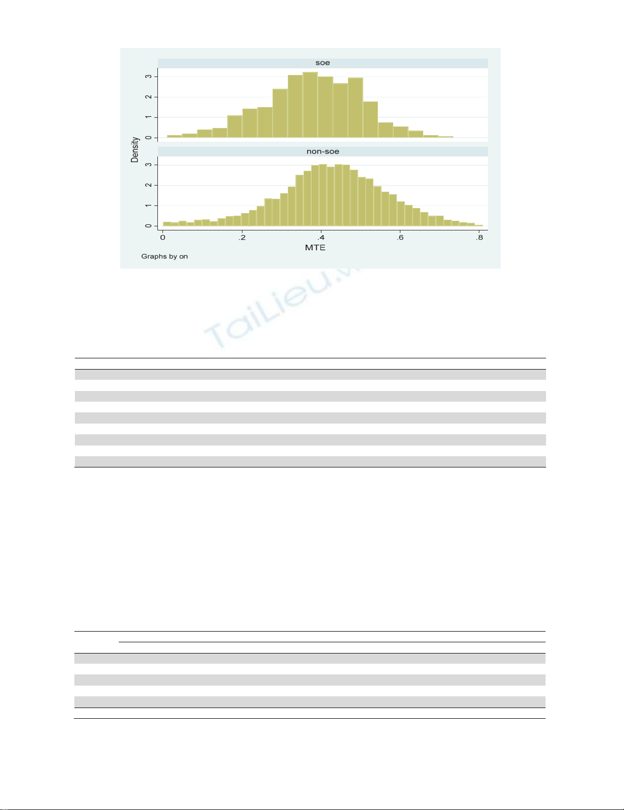
The MTE for SOE and for non-SOE are depicted in Fig. 1
T. M. Nguyen et al. / Decision Science Letters 8 (2019)
229
Fig. 1. The MTE for SOE and for non-SOE firms in 2016
From Fig. 1, it can be seen that the technical efficiency for both soe and non-soe firms are fairly low:
around 50% of firms have MTE less than 0.5. Table 3 shows the numbers in more details:
Table 3
MTE for SOE and for non-SOE in different percentiles, accumulated (in percentage)
MTE SOE non-SOE
0-0.1 1.6 2.3
0.1-0.2 8.6 6.3
0.2-0.3 23.5 16.8
0.3-0.4 56.1 41.1
0.4-0.5 84.3 70.3
0.5-0.6 97.4 89.4
0.6-0.7 99.7 97.5
0.8-0.9 100.0 100.0
0.9-1.0 100
Source: calculated from Enterprise census.
Table 3 shows that the number in column SOE is always greater than that in non-SOE column, except
for the first value. It implies that the non-SOE firms perform better than SOE firms in terms of technical
efficiency, for example, 97.4 % of SOE firms have MTE < 0.6, while the number for non-SOE firms
is 89.4%.
Result for technology gap ratio
For the technology gap ratio, we also wish to look at more details for each sub-industry. The technology
gap ratios for SOE and non-SOE firms for each sub-industry are reported in Table 4.
Table 4
Technology gap ratio by ownership and by sub-industry.
Interval Foo
d
Weavin
g
Cloths chemical electronics
Soe non-soe soe non-soe soe non-soe soe non-soe soe non-soe
0-0.2 0.98 0.00 1.35 0.00 0.00 0.00 0.00 0.00 0.00 0.00
0.2-0.4 7.35 0.00 9.46 0.00 4.00 0.00 21.15 0.00 14.29 0.00
0.4-0.6 21.08 0.00 24.32 0.00 32.00 0.00 38.46 0.00 57.14 0.00
0.6-0.8 40.69 10.20 36.49 15.35 40.00 3.85 30.77 19.22 28.57 35.90
0.8-1 29.90 89.80 28.38 84.65 24.00 96.15 9.62 80.78 0.00 64.10
Total 100 100 100 100 100 100 100 100 100 100
Source: calculated from Enterprise census


![Kinh tế vi mô: Giới thiệu chương 1 [Tổng quan kiến thức]](https://cdn.tailieu.vn/images/document/thumbnail/2011/20111230/dungtranktgt/135x160/giao_trinh_kinh_te_hoc_vi_mo0001_0349_0071.jpg)


