ISSN 1859-1531 - THE UNIVERSITY OF DANANG - JOURNAL OF SCIENCE AND TECHNOLOGY, VOL. 22, NO. 11C, 2024 109
SHORT-TERM PREDICTION OF REGIONAL ENERGY CONSUMPTION BY
METAHEURISTIC OPTIMIZED DEEP LEARNING MODELS
Ngoc-Quang Nguyen*, Phuong-Thao-Nguyen Nguyen, Quynh-Chau Truong
The University of Danang - University of Science and Technology, Viet Nam
*Corresponding author: nnquang@dut.udn.vn
(Received: September 26, 2024; Revised: October 11, 2024; Accepted: October 12, 2024)
DOI: 10.31130/ud-jst.2024.567E
Abstract - Modern civilization is heavily dependent on energy,
which burdens the energy sector. Therefore, a highly accurate
energy consumption forecast is essential to provide valuable
information for efficient energy distribution and storage. This study
proposed a hybrid deep learning model, called I-CNN-JS, by
incorporating a jellyfish search (JS) algorithm into an ImageNet-
winning convolutional neural network (I-CNN) to predict week-
ahead energy consumption. First, numerical data were encoded into
grayscale images for input of the proposed model, showcasing the
novelty of using image data for analysis. Second, a newly
developed metaheuristic optimization algorithm, JS, was used to
improving model accuracy. Results showed that the proposed
method outperformed conventional numerical input methods. The
optimized model yielded a mean absolute percentage error
improvement of 0.5% compared to the default models, indicating
that JS is a promising method for achieving the optimal
hyperparameters. Sensitivity analysis further evaluated the impact
of image pixel orientation on performance model.
Key words - short-term prediction; energy consumption; deep
learning; convolutional neural network; metaheuristic
optimization; machine learning; time-series deep learning
1. Introduction
The energy sector plays a vital role in the global
economy, directly affecting industries, infrastructure, and
social life. Ensuring a stable power supply helps minimize
negative impacts on production and business while
supporting the promotion of industrialization,
modernization, and sustainable development. Forecasting
energy consumption is one of the core factors in the
effective management of the energy system, especially in
the context of increasing scale and volatility in energy
consumption [1].
However, with the increasing integration of renewable
energy sources into the grid, the instability of the energy
supply has become a challenge. The completely
unpredictable nature of sources such as wind and solar,
combined with the ever-changing demand, requires
accurate forecasting tools to support system operators in
decision-making. Therefore, forecasting energy
consumption has become a vital task to optimize energy
distribution, ensuring economic efficiency and
sustainability of the energy system [2].
Traditional methods such as linear regression, time-
based statistical models, or simple machine learning (ML)
techniques have been widely used for many years to forecast
energy consumption [3-5]. However, with the development
of technology and the abundance of data, these methods are
gradually becoming limited when faced with complex and
highly nonlinear energy models [6]. Deep learning (DL) has
emerged as a potential solution due to its ability to learn and
model complex relationships in data. DL can exploit
information from large, multidimensional datasets to
forecast energy consumption more accurately [7].
One of the most widely used DL models is the
convolutional neural network (CNN), thanks to its ability
to capture spatiotemporal relationships as well as time
series features [8]. However, implementing DL models for
energy consumption forecasting also faces significant
challenges, the most important of which is the parameter
optimization process. DL models often require configuring
parameters such as the number of layers, the number of
nodes in each layer, and other hyperparameters, which
directly affect the accuracy and performance of the model.
Optimizing these parameters is often done by trial and error
methods or simple optimization algorithms, but they do not
always guarantee optimal performance for the model.
To improve this optimization, hyperparameter
optimization algorithms have been applied to optimize
hyperparameters and enhance the performance of deep
learning models. These optimization algorithms are
designed to search large parameter spaces, avoiding falling
and local minima, a common problem in traditional
optimization methods, while providing more flexible and
efficient model tuning.
Although DL models have been applied in various
fields, such as image processing, natural language
processing, and medicine, their application in the field of
short-term energy consumption forecasting is still limited
and underexploited. Therefore, this study aims to bridge
this gap by proposing a method that combines I-CNN
models and metaheuristic optimization algorithms for
regional energy consumption forecasting.
Specifically, this study will focus on:
1) Proposing a hybrid DL model based on I-CNN and
JS algorithm to predict energy consumption.
2) Developing an automated process to convert
numerical data into images as input for I-CNN.
3) Conducting sensitivity analysis to examine the effect
of image pixel orientation on model accuracy.
2. Related works
2.1. Convolutional neural network
Convolutional neural networks (CNNs) are a type of
artificial neural network specifically designed to process
110 Ngoc-Quang Nguyen, Phuong-Thao-Nguyen Nguyen, Quynh-Chau Truong
data with a grid structure, such as images and videos.
CNNs are widely used in computer vision, such as object
recognition, image classification, face recognition, and
video analysis. Unlike traditional models that require
manual feature extraction, CNNs automatically learn
features from raw data, especially spatial features, through
the structure of filters.
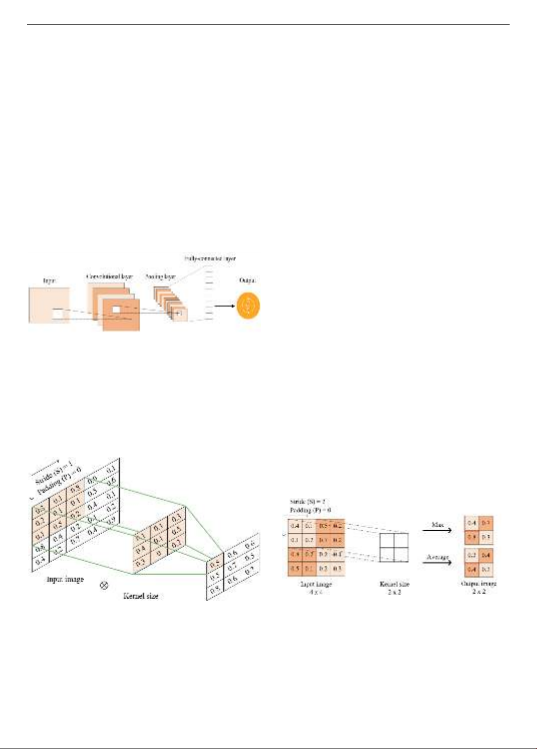
The basic architecture of CNN typically consists of an
input layer that receives an input image, and several hidden
layers that include three different layers: a convolutional
layer, a pooling layer, a fully-connected layer, and an
output layer that produces the final output. Figure 1
displays a simple CNN architecture. CNN becomes more
and more complicated as it progresses from the
convolutional layer to the FC layer. Thanks to such an
arrangement, CNN can first recognize simpler patterns
(lines, curves) and then more complicated features (faces,
objects) of an image before fully recognizing the pattern
and extracting the useful features.
Figure 1. The architecture of a CNN
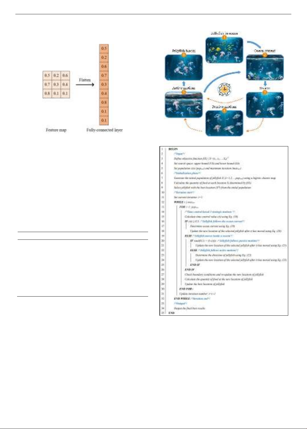
The convolutional layer is one of the main and most
characteristic components of a CNN, which helps extract
features from input data, especially images. The
convolutional layer uses one or more filters (also known as
kernels). These filters are small matrices whose values are
learned during training. The filter is passed through the
entire input image, calculating the convolution between the
filter and the corresponding regions of the image, and
creating a feature map.
Figure 2. Convolution operation of the convolution layer
The convolution operation (Figure 2) multiplies each
element of the filter by the corresponding part of the image,
then sums it up and outputs a new value. This calculation
continues as the filter moves through the entire image. The
result of this process is a feature map that is smaller or
equal to the original image, depending on parameters such
as stride, and padding. The convolution operation can be
defined as follows:
𝐶𝑖= 𝑏𝑖+𝐼𝑗𝐹𝑖𝑗
𝑑𝑖
𝑗=1 , 𝑖 = 1𝑑𝑐 (1)
where, 𝐶𝑖 is the output of convolutional layer or feature
map of size (𝑐𝑤 𝑥 𝑐) in which (𝑐𝑤 𝑥 𝑐)= ((𝑣𝑤𝑟𝑤
2𝑝)/𝑠+1)𝑥((𝑣𝑟2𝑝)/𝑠+1) (𝑣𝑤,𝑣are the width
and height of input volume, 𝑟𝑤,𝑟 are the width and height
of receptive field size, p is the amount of zero padding used
on the border, s is the stride with which they are applied),
𝐵𝑖 is the bias, 𝑑𝑖 is the depth of input, 𝐼𝑗 is the input image,
𝐹𝑖𝑗 is the filter, and 𝑑𝑐 is the depth of convolutional layer.
After convolution, the values in the feature map are
usually passed through an activation function such as
ReLU to nonlinearize, retain important features, and ignore
negative values that are not meaningful to the model. The
general formula of the activation function can be defined
as follows:
𝑌𝑖= 𝑓(𝐶𝑖) (2)
where, 𝑌𝑖 is the output of the convolutional layer after
applying the activation function and f is the activation
function.
Pooling layer in CNN is a downsampling layer used to
reduce the size of feature maps without losing too much
important information. Pooling reduces the number of
parameters and computations in the network, while
increasing the resistance to changes in the location of
features in the input data, making the model more robust to
local changes in the image. The dimensions of the output
obtained from the pooling layer are as follows:
(𝑐𝑤𝑓𝑤+ 1)/𝑠 𝑥 (𝑐𝑓+1)/𝑠 𝑥 𝑐𝑛 (3)
where, 𝑐𝑛 is the number of channels in the feature map and
𝑓𝑤 𝑥 𝑓 is the width and height of the filter.
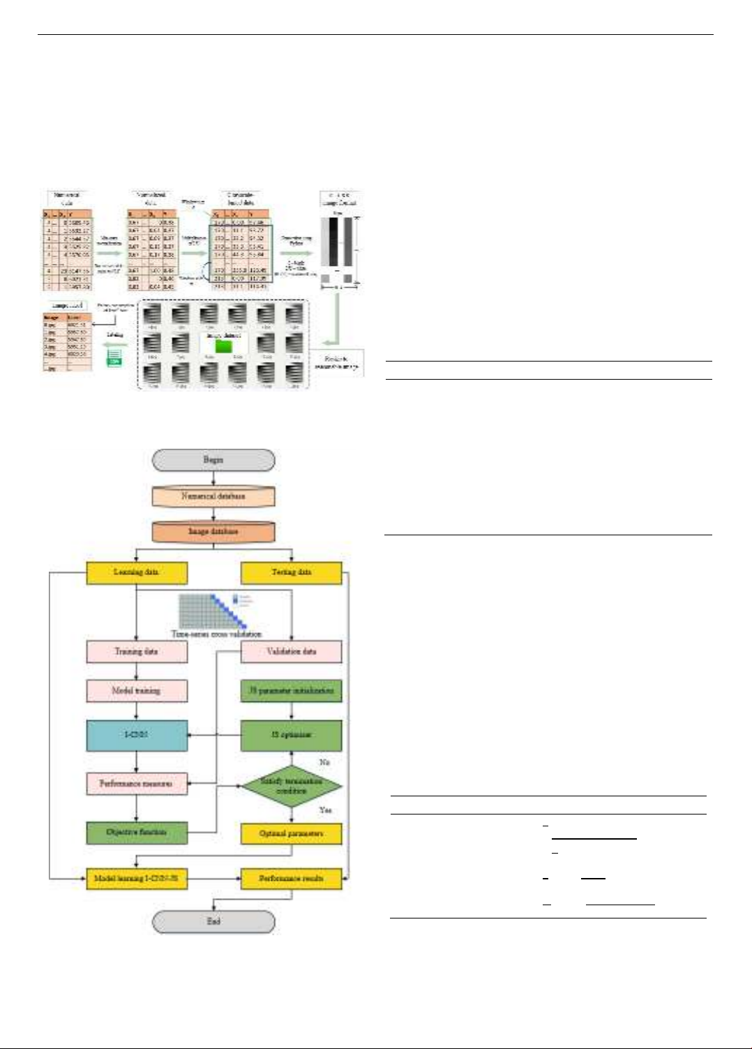
Average pooling and max pooling are two typical pooling
approaches. Max pooling is the most common type in CNN
networks, which selects the largest value in each small region
of the feature map. Instead of selecting the largest value,
average pooling averages the values in the small regions. This
is less commonly used than max pooling but still has
applications in some cases. Figure 3 presents the illustration
of max pooling and average pooling.
Figure 3. Max pooling and average pooling
A fully-connected (FC) layer is a layer in which each
neuron is connected to all the neurons in the previous layer.
It is the final component of CNN and is often used to
perform tasks such as classification or prediction. After
previous layers, such as convolutional and pooling layers,
have extracted local features from the data, the FC layer
aggregates and processes all of this information, allowing
the network to learn more complex features from the entire
data. In classification models, the FC layer is typically at
ISSN 1859-1531 - THE UNIVERSITY OF DANANG - JOURNAL OF SCIENCE AND TECHNOLOGY, VOL. 22, NO. 11C, 2024 111
the end of the network and has as many neurons as there
are labels to classify. In prediction tasks, the FC layer can
predict continuous values, such as in regression problems.
Figure 4 presents the structure of the FC layer.
Figure 4. Structure of a fully-connected layer
2.2. ImageNet-winning convolutional neural network
The ImageNet Large Scale Visual Recognition
Challenge (ILSVRC) is one of the most prestigious
competitions in the field of computer vision, especially in
object recognition in images. The winning CNN models in
this competition have driven significant advances in
computer vision technology. Several popular CNN
architectures have been developed that differ in their
approach and have significantly improved not only the
accuracy but also the efficiency of the model on various
tasks compared to their predecessors. Table 1 shows the I-
CNN architectures used in this study.
Table 1. Overview of I-CNN structures used in this study
Attribute
Parameters (million)
Size (MB)
VGG19
143.7
549
ResNet50V2
25.6
98
Inceptionv3
23.9
92
MobileNetV2
3.5
14
DenseNet201
20.2
80
NASNetLarge
88.9
343
EfficientNetB0
5.3
29
ConvNeXtTiny
-
28.6
2.3. Jellyfish Search Algorithm
The JS algorithm is a metaheuristic optimization
algorithm inspired by the migration and hunting behavior of
jellyfish in the ocean, proposed by Chou et al. in 2020 [9].
The algorithm simulates the two main movements of
jellyfish: random movements as they drift with the ocean
currents and directional movements as they swim in search
of food sources. Combining the exploration and exploitation
of the search space, JS optimizes complex problems by
balancing between exploring new regions and exploiting
potential solutions, avoiding getting stuck in local extrema.
JS has been successfully applied to various
optimization problems, from continuous space
optimization to discrete optimization, and the results show
that JS can achieve higher efficiency and faster
convergence than traditional algorithms. In addition, the
algorithm does not require many complex parameters. The
flowchart and pseudocode of the JS algorithm are shown in
Figures 5 and 6 respectively.
Figure 5. Jellyfish behavior in the ocean
Figure 6. Pseudocode of the jellyfish search algorithm
3. Proposed I-CNN-JS algorithm
3.1. Image conversion process
This study proposes a numerical-to-image data
conversion method that allows the use of image processing
and computer vision techniques to implement I-CNN
models. Each time step is represented as a pixel in the
image, enabling the model to capture spatial relationships
between different time steps, correlations, and
dependencies to identify geographically close regions and
detect similar patterns in energy consumption, which are
difficult to discern from raw digital data alone.
The image conversion process is detailed in Figure 7.
112 Ngoc-Quang Nguyen, Phuong-Thao-Nguyen Nguyen, Quynh-Chau Truong
Initially, n attributes of each observation are used to
generate a n × 1 grayscale image. These initial images are
processed using a sliding window technique with a window
size of k to generate a n+1 × k grayscale image. First, min-
max normalization is performed to scale the numerical data
to values between 0 and 1. Then, the normalized data is
multiplied by 255 and encoded into images with grayscale
values between 0 and 255. Finally, each image is labeled
with the k + mth energy consumption data.
Figure 7. The conversion of numerical data into
grayscale images
3.2. I-CNN-JS algorithm
Figure 8. The proposed optimized hybrid model
The proposed I-CNN-JS algorithm, which combines
the I-CNN architecture with the JS algorithm, not only
aims to leverage the power of the I-CNN architectures in
predicting energy consumption but also can find the global
optimal solution to improve prediction accuracy. The
process of the I-CNN-JS algorithm is depicted in Figure 8.
4. Result analysis
4.1. Dataset and parameter setting
This study collected five-year hourly energy
consumption data from 2019 to 2023 from a power
company by using the Data Miner tool on the PJM website
(https://www.pjm.com/). This dataset includes 43,824 data
points after the kNN imputation method was used to handle
missing data during the data collection.
Table 2 presents the attributes of the energy
consumption dataset used in this study. The time index was
decomposed into time-series characteristics X1-X7 such as
hour, month, quarter, year, day of the week, day of the
month, and day of the year which were used to predict
energy consumption Y.
Table 2. Attributes of the dataset
Attribute
Description
Time Index
Time data are recorded
Month
Month (1, 2, …, 12)
Quarter
Quarter (1, 2, …, 4)
Year
Year (2019, 2020, …, 2023)
Hour
Hours (0, 1, …, 23)
Day of week
Day (0, 1, …, 6)
Day of month
Day (0, 1, …, 31)
Day of year
Day (0, 1, …, 366)
Energy consumption
Energy consumption (MWh)
4.2. Validation and performance evaluation
The dataset was divided into 80% for learning (from
2018 to 2022) and 20% for testing (2023). The learning
dataset was then divided into 85% and 15% for training and
validation, respectively. This study uses the time-series
cross-validation method, which divides the data in time
order, ensuring that future data points are not used to predict
past data to preserve the sequentiality of the data [10].
Five widely used regression metrics including the mean
absolute error (MAE), root mean square error (RMSE),
mean absolute percentage error (MAPE), training time, and
synthesis index (SI) were used to evaluate and validate
model performance. Table 3 presents the equation of these
performance metrics.
Table 3. Performance measures
Performance measures
Equation
MAE
1
𝑛 |𝑦𝑖𝑦𝑖|
𝑛
𝑖=1
RMSE
1
𝑛(𝑦𝑖𝑦𝑖)2
𝑛
𝑖=1
MAPE
1
𝑛|𝑦𝑖−𝑦
𝑖
𝑦𝑖|
𝑛
𝑖=1
SI
1
𝑚(𝑃𝑖−𝑃(𝑚𝑖𝑛,𝑖)
𝑃(𝑚𝑎𝑥,𝑖)−𝑃(𝑚𝑖𝑛,𝑖))
𝑚
𝑖=1
where, 𝑛 is the number of predictions, 𝑦𝑖 the predicted
value; 𝑦𝑖 is the actual value, 𝑚 is the number of
performance metrics, 𝑃𝑖 is the value of the performance
metric, 𝑃(𝑚𝑎𝑥,𝑖) is the maximum value of performance
metric, and 𝑃(𝑚𝑖𝑛,𝑖) is the minimum value of performance
ISSN 1859-1531 - THE UNIVERSITY OF DANANG - JOURNAL OF SCIENCE AND TECHNOLOGY, VOL. 22, NO. 11C, 2024 113
metric. Their lower values indicate better performance.
4.3. Model establishment
A typical CNN structure normally includes a softmax
activation function at the end of the network for
classification tasks. However, predicting energy
consumption is a regression task. Therefore, the CNN
models in this study were restructured by replacing the
softmax activation function in the final layer with a linear
activation, which allows the network to output continuous
values rather than probabilities.
While CNN, LSTM, and GRU models were deployed
using the Keras library in Python, ML models were
constructed in Scikit-learn and XGBoost in Python. Table
4 presents the performance results of predictive models for
week-ahead energy consumption.
Table 4. Performance result of models for week-ahead
energy consumption
Model
RMSE
(kWh)
MAPE
(%)
SI
t
(h)
VGG19
421.6
8.1
(8)
1.52
ResNet50V2
387.1
7.5
(5)
1.23
Inceptionv3
413.1
7.9
(7)
1.22
MobileNetV2
393.6
7.6
(4)
1.02
DenseNet201
383.2
7.4
(3)
1.19
NASNetLarge
397.5
7.7
(6)
1.48
EfficientNetB0
368.9
7.3
(2)
1.00
ConvNeXtTiny
355.2
7.1
(1)
1.00
ANN
774.0
11.2
(13)
0.08
RF
762.5
10.9
(12)
0.09
SVR
787.6
11.4
(14)
0.08
XGBoost
686.9
10.3
(11)
0.08
LSTM
691.6
10.2
(10)
0.16
GRU
680.8
9.9
(9)
0.15
Note: kWh: kilowatt hours
The results revealed that ConvNeXtTiny, XGBoost, and
GRU were the best-performing models in their categories in
predicting week-ahead energy consumption, with MAPE
values of 7.1%, 10.3%, and 9.9%, respectively. Notably, all
CNN models provided more accurate predictions than the
rest with the MAPE range from 7.1% to 8.1%, occupying
the top 8 out of 14 models according to the SI index, in which
ConvNeXtTiny is the best model. This impressive result
demonstrated that the proposed model outperforms methods
using numerical data.
The running time shows that the CNN models in this
study take significantly longer than other numerical
models. For example, the CNN model takes more than one
hour to predict energy consumption, while the numerical
models only take about 0.8 to 0.9 hour for the ML models
and 0.15 to 0.16 hour for the time-series DL models.
Although CNN models provide better prediction
results, users should choose the model based on their goals,
usage context, and computational resources. For example,
CNN models should be used in cases where accurate
predictions are required for research and measurement
purposes, where high accuracy is the top factor and longer
computation times are accepted. In contrast, numerical
models such as GRU are more suitable for real-time
predictions, where the balance between accuracy and speed
is important.
4.4. Optimization
A validation of the power of optimization algorithms,
namely Jellyfish Search, and two well-known
metaheuristic algorithms, Teaching-Learning-Based
Optimization (TLBO) and Symbiotic Organisms Search
(SOS), was performed before incorporating one of them
into the best model for parameter optimization. Ten
benchmark functions were selected to validate the
effectiveness of these algorithms, namely Step, Trid10,
Zakharov, Foxholes, Michalewicz2, Shubert, Ackley,
Langermann2, and Fletcher Powell10. Hit rate, the ratio
between the number of times the algorithm produces the
optimal result and the number of times the independent
optimization is performed, and the running time were used
to compare the effectiveness of the algorithms.
The results in Table 5 show that JS outperforms SOS
and TLBO in both hit rate and computation time. The hit
rate of JS is 100%, which is 31.02% and 27.88% higher
than SOS and TLBO. As for running time, JS only needs
11.02 seconds to find the optimal values of the benchmark
functions, while the figures for SOS and TLBO are 63.69
and 62.96, respectively. Therefore, JS was then selected as
the best optimization algorithm incorporated into the
ConvNeXtTiny model.
Table 5. Comparison results of benchmark functions in the
optimization algorithms
Criteria
JS
SOS
TLBO
Hit rate (%)
100
68.98
72.12
Running time (sec)
11.02
63.69
62.96
Table 6 shows the results of the model performance
before and after optimization. The results demonstrate that
JS is effective in improving the accuracy of the model, with
MAPE improving by 0.5% compared to the original model.
Table 14 shows the parameters after optimization.
Table 6. Comparison results of model performance before and
after optimization
Model
MAE
(kWh)
RMSE
(kWh)
MAPE
(%)
I-CNN (ConvNeXtTiny)
352.1
355.2
7.1
I-CNN (ConvNeXtTiny) - JS
334.2
336.2
6.6
4.5. Sensitivity analysis of image pixel order
Another numerical experiment was conducted based on
the ConvNeXtTiny model to investigate the influence of
image orientation on prediction accuracy. Two types of
image orientations, including the original pixel array
(randomly arranged) and the pixel array arranged
according to the correlation between input attributes and
energy consumption were adopted in this study.
Specifically, the image data was reformatted in three ways:
arranging the pixels randomly, arranging them in
ascending order, and descending order based on the
correlation value.
Table 6 presents the results of the sensitivity analysis of
image orientation on the prediction model accuracy. It can