Transport and Communications Science Journal, Vol. 76, Issue 01 (01/2025), 31-41
31
Transport and Communications Science Journal
CONVOLUTIONAL NEURAL NETWORK FOR DETERMINING
THE FLOW FIELD AROUND AN AIRFOIL AND BLUNT-BASED
MODELS
Tran The Hung*
Faculty of Aerospace Engineering, Le Quy Don Technical University, No 236 Hoang Quoc
Viet Street, Bac Tu Liem, Hanoi, Vietnam
ARTICLE INFO
TYPE: Research Article
Received: 05/06/2024
Revised: 24/10/2024
Accepted: 10/01/2025
Published online: 15/01/2025
https://doi.org/10.47869/tcsj.76.1.3
* Corresponding author
Email: tranthehung_k24@lqdtu.edu.vn; Tel: +84355544745
Abstract. The convolutional neural network is widely applied in the classification of images
and medicine. Some current networks are used in aerospace engineering and show a high
potential in determining aerodynamic forces and flow fields. This article constructs a
convolutional neural network for predicting pressure and velocity fields around a two-
dimensional aircraft wing model (airfoil model). Training data is computed using the
Reynolds-averaged method, and then extracted, focusing on the flow around the wing. Input
data includes geometric parameters, and airfoil inlet velocity, and output data includes
pressure field and flow velocity around the airfoil. The convolutional neural network is based
on improving the U-Net network model, commonly used in medical applications. The results
show that the convolutional neural network accurately predicts flow around the airfoil, with
an average error below 3%. Therefore, this network can be used and further developed to
predict flow around the wing. The network is then applied to predict the pressure and pressure
fields around a blunt-based model with different aspect ratios. The main feature of the flow
can be extracted from the network. Results related to pressure distribution, velocity, and
method error are presented and discussed in the study. This study also suggests improving the
network and applying it to pressure and velocity fields in aerospace engineering.
Keywords: Convolutional neural network, U-Net, airfoil, blunt-based model, flow fields,
pressure, velocity.
@ 2025 University of Transport and Communications
Transport and Communications Science Journal, Vol. 76, Issue 01 (01/2025), 31-41
32
1. INTRODUCTION
Over the past century, the aircraft wing has remained a pivotal component for generating
lift, which is crucial for flight in the atmosphere. With advancements in aviation and
computational methodologies, wing database systems have been continually enhanced.
Prominent examples include the NACA wing system and Xfoil software, which swiftly
provide data on lift, drag, and pressure distribution on the wing surface [1]. More precise
techniques, such as utilizing software to tackle finite volume problems, enable comprehensive
analysis of pressure, velocity, and friction around the wing surface, rooted in classical
mathematical equations and computational space discretization [2,3].
In contemporary times, artificial neural networks have gained widespread application
across scientific and engineering domains. Leveraging substantial training datasets, neural
networks yield predictions with minimal errors compared to conventional methods. In
aerodynamics, artificial neural networks are employed to forecast the lift and drag values of
models. Global networks like convolutional neural networks facilitate the precise distribution
of pressure and velocity fields around models with minimal errors. This methodology
involves generating training and testing data from traditional computational approaches, and
then restructuring them into four-dimensional arrays. Subsequently, the data undergoes
convolutional neural network processing to extract features, which are then reconstructed into
pressure and velocity fields. Throughout the training phase, network parameters are fine-tuned
to yield pressure and velocity field results resembling the original data. Various networks
have been developed for this task, such as FlowNet for optical flow and U-Net for medical
applications [4]. However, it's worth noting that artificial neural networks, beyond their
mathematical foundations, possess architectural nuances, influencing the outcome based on
the chosen convolutional network design.
Another difficult task is from prediction of the flow field around the blunt base model.
This model features a large separation flow at the base, which results in a low-velocity region
and high aerodynamic drag [5]. Building a network for prediction flow around the blunt body
is also an important task, which was not been conducted before. It is also interesting to know
how much is the accuracy of the current network in predicting the pressure and velocity fields
around the blunt-base model.
In this research, we suggest alterations to the conventional U-Net architecture to facilitate
the extraction of pressure and velocity fields surrounding a two-dimensional aircraft wing
model (airfoil). Our dataset comprises 400 airfoil instances with varied shapes and flow
conditions for both training and testing. Our findings from training the U-Net model
demonstrate its capability to predict velocity and pressure field characteristics with high
accuracy, exhibiting a typical error rate of under 3%. Thus, these modified networks hold
promise for computational fluid dynamics applications concerning physical model analysis.
2. CONVOLUTIONAL NEURAL NETWORK DIAGRAM AND TRAINING DATA
2.1. Convolutional neural network diagram
U-Net Convolutional Neural Network is a network architecture used in the field of image
processing, particularly for segmentation tasks [4] [6] [7]. It was also used by Wu et al. [8] for
detection of the infrared object. This architecture is designed to retain high-level information
(learned from convolutional layers) while also maintaining specific positional information
Transport and Communications Science Journal, Vol. 76, Issue 01 (01/2025), 31-41

33
(learned from pooling layers). U-Net is typically divided into two main parts: the encoder and
the decoder. The encoder uses convolutional layers to extract information from the input
image and applies pooling layers to reduce the feature size while retaining important
information. Conversely, the decoder uses transposed convolutional layers to reconstruct the
image with high resolution and combines information from the corresponding encoding layers
through skip connections to recreate specific objects. U-Net has demonstrated good
performance in various applications, including cell segmentation in medical images, object
recognition in images, and many other tasks. The unique structure of U-Net allows it to retain
both high-level and positional information, making it a popular choice for tasks that require
both detailed and positional information about objects. The output results depend on the
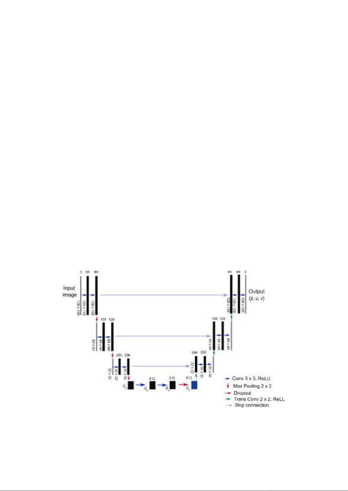
number of layers in the U-Net. For the airfoil models, this study uses a U-Net with three
input-output layers. Additionally, in comparison to the previous study by Du et al [4], the
network is redesigned by us for a suitable application of the airfoil model. By reducing the
number of layers, the parameters of the network are reduced and the training process becomes
faster. The network input is modified to be a three-dimensional matrix of size 128×128×3.
The size of the image is also modified for the current study. The first two dimensions
represent the image size, and the third dimension sequentially represents the model's
geometry, the input velocity in the x direction, and the input velocity in the y direction. Each
convolutional layer is followed by a ReLU layer, and the final convolutional layer is followed
by a Max Pooling layer. Initially, the U-Net network was used for image segmentation.
Therefore, the output parameter is changed to a three-dimensional matrix of size 128×128×3,
where the third dimension sequentially represents the pressure field, the output velocity in the
x direction, and the output velocity in the y direction. The network includes 7.6 million
parameters. The structure of the U-Net and its parameters are presented in Figure 1. The
network structure and training process are built using MATLAB software. Previously, Du et
al [4] used Python and many processes for the training. In this study, we create a program, so
all parameters and their effect on the results can be controlled.
Figure 1. Diagram of the 3-layer U-Net network.
Transport and Communications Science Journal, Vol. 76, Issue 01 (01/2025), 31-41
34
2.2. Training Data
The training data used in this study is taken from the dataset published by Thuerey and
colleagues [6]. Specifically, the Reynolds-Averaged Navier-Stokes (RANS) method with the
Spalart-Allmaras turbulence model is used. The model was developed by Spalart and
Allmaras [9], which uses one additional equation for predicting turbulent eddy viscosity. The
equation for the model is shown in Eq. (1). The biggest advantage of the Spalart-Allmaras
model is that the simulation is fast and the requirement of y+ is not strong. Consequently, it is
widely used in fluid mechanics in the initial aerodynamic designing process [10].
2
1
1 2 1 2 2
2
ˆ ˆ ˆ ˆ ˆ ˆ
1
ˆˆˆ
1b
j b t t b
j j j i i
c
u c f S c f f c
t x d x x x x









 





(1)
Where the turbulent eddy viscosity is calculated by:
1
ˆ
tv
f

with
3
133
1
v
v
fc
and
ˆ
. Here, ρ is air density, ν is kinematic viscosity and
μ is the dynamic viscosity. Additional definitions are given by the following:
with
2ij ij
WW
and
2
1
11
v
v
ff

,
1/6
6
3
66
3
1c
fg
gc



6
2
g r c r r
,
22
ˆ
min ,10
ˆ
rSd



,
2
2 3 4
exp( )
t t t
f c c

,
1
2
j
i
ij
ji
x
x
Wxx






The other constant parameters are selected as:
cb1 = 0.1355, σ = 2/3, cb2 = 0.622, κ = 0.41, cω2 = 0.3, cω3 = 2, cv1 = 7.1, ct3 = 1.2, ct4 = 0.5 and
12
12
1
bb
cc
c


.
Calculations are performed in the OpenFoam environment. The geometric features and
the flow around the model are cropped to a size of 128 × 128 pixels to facilitate the training
process. Note that since a MATLAB program is used, the size of each node is the same for
points close and far from the models. Consequently, the boundary layer cannot be captured
for the training data. A total of 400 data sets are used for training. The angle of attack is
changed from -22.5° to 22.5°. The Reynolds number is in the range of 0.5-5.0 million.
Consequently, separation flow can occur on the surface, and training data contains different
flow types. The velocity was then normalized by freestream velocity while the pressure was
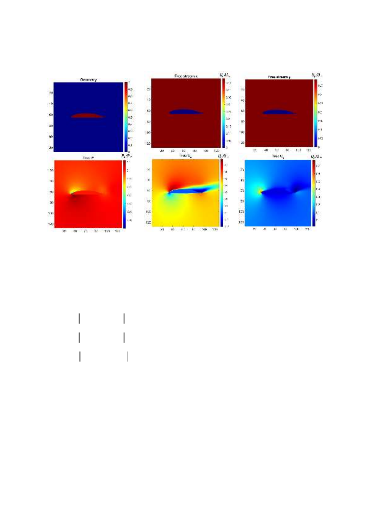
normalized by static pressure before training. An example of the training data field is shown
in Figure 2. Here, the x and y axes present the pixel number and the flow is from the left to
right. It includes the geometry, the free stream in x and y directions, the results of pressure
fields, and velocity fields. All data of the input and output has the same size of 128 × 128
pixels. Note that this data was generated by Thuerey and colleagues [6] with detailed
validation. Here, we can see that the numerical method can simulate well the flow
phenomenon around the airfoil model such as the separation flow on the trailing edge, a high
pressure and low velocity around the leading edge. However, since the data in MATLAB is
Transport and Communications Science Journal, Vol. 76, Issue 01 (01/2025), 31-41
35
organized as a matrix, the boundary layer may not be captured well in the simulation.
Consequently, it can be confirmed that the training data is reliability.
Figure 2. Training data for the training process.
2.3. Training Model
The three-layer U-Net network described in section 2.1 is used for the training process.
The airfoil data is divided into 80% for training and 20% for testing. The training data is
divided into mini-Batch with a size of 10. The loss function is calculated as the average error
of the pressure field and velocities during training with the standard data. The loss function of
is determined by Eq. (2):
,,
()
x x True x Pridict
Loss P P P
(2)
,,
()
x x True x Pridict
Loss V V V
,,
()
x x True x Pridict
Loss U U U
( ) ( ) ( )
xy
Loss mean Loss P Loss U Loss U
Note that the loss function by Equation (2) was often used for training process of
aerodynamic qualities, previously. A total of 100 epochs are performed for the training
process. The adaptive moment estimation (Adam) algorithm is used. The learning rate is fixed
at 0.001. It should be noted that the learning rate can affect the convergence of the problem.
However, calculations in this study show that reducing or changing the learning rate around
the chosen parameter does not significantly change the loss function. Additionally, four, and
five-layer U-Net were also attempted in predicting the pressure and velocity fields. However,
the training time increases while the results are not improved. Consequently, a three-layer