Dự báo nhu cầu bằng Deep Learning cho công ty FMCG Việt Nam

Applying deep learning to forecast the demand of a Vietnamese FMCG companyLe Duc Dao* and Le Nguyen KhoiHo Chi Minh City University of Technology, Vietnam Naonal University, VietnamABSTRACT In the realm of Fast-Moving Consumer Goods (FMCG) companies, the precision of demand forecasng is essenal. The FMCG sector operates in a highly uncertain environment marked by rapid market shis and changing consumer preferences. To address these challenges, the applicaon of deep learning techniques, parcularly Long Short-Term Memory (LSTM) networks, has emerged as a vital soluon for enhancing forecast accuracy. This research paper focuses on the crical role of demand forecasng in FMCG, emphasizing the need for LSTM-based deep learning models to deal with demand uncertainty and improve predicve outcomes. Through this exploraon, we aim to illuminate the link between demand forecasng and advanced deep learning, enabling FMCG companies to thrive in a highly dynamic business landscape.Keywords: demand forecast, ARIMA, deep learning, long-short term memory, FMCGWithin the domain of Fast-Moving Consumer Goods (FMCG), the importance of precise demand predicon remains of paramount signiﬁcance [1]. The nature of the FMCG industry is represented by swi market ﬂuctuaons and ever-shiing consumer preferences. As product life cycles grow ever shorter and consumers become familiar with greater product variety, FMCG companies face increasing pressure to accurately ancipate future demand in order to opmize producon schedules, inventory levels, supply chain coordinaon, promoonal campaigns, workforce allocaon, and other key operaons that can make proﬁt for them. However, the complex factors inﬂuencing product demand in the FMCG space oen proves diﬃcult to model using tradional stascal techniques. Demand drivers may include broad economic condions, consumer conﬁdence, compeve landscape, channel dynamics, weather paerns, commodity prices, cultural trends, and a myriad of other variables that can be diﬃcult to quanfy. While ARIMA (Autoregressive Integrated Moving Average) and other tradional forecasng techniques have been valuable tools for predicon in various ﬁelds, they oen struggle to cope with the complexies of today's rapidly changing and highly dynamic world [2]. Such methods rely heavily on historical sales paerns connuing into the future. When condions or consumer preferences shi suddenly, tradional models fail to account for new realies. Consequently, the adopon of advanced deep learning methodologies, parcularly the Long Short-Term Memory (LSTM) networks, has gained prominence as an essenal method for improving the precision of forecasts [3]. LSTMs and related recurrent neural network architectures possess provide advantages in processing me series data, idenfying subtle paerns across long me lags, and adapng predicons based on newly available informaon. Inspired by the workings of human memory, LSTM models can learn context and discard outdated assumpons in light of updates, much as a supply chain manager would aer nocing an impacul new trend. By combining the basic stascal foundaon of methods like ARIMA with the paern recognion capabilies of deep learning, FMCG forecasng stands to become signiﬁcantly more accurate and responsive to ﬂuctuaons in consumer demand. Stems from the fact that ARIMA's ability to model linear historical paerns and LSTM's ability for uncovering nonlinear relaonships, a combined forecast of ARIMA and LSTM were proposed to guide the direcon of this research, considering the nature of products. Further invesgaons into opmal model architectures, hyperparameter tuning, and 85Hong Bang Internaonal University Journal of ScienceISSN: 2615 - 9686 DOI: hps://doi.org/10.59294/HIUJS.VOL.5.2023.552Hong Bang Internaonal University Journal of Science - Vol.5 - 12/2023: 85-92Corresponding author: Le Duc DaoEmail: lddao@hcmut.edu.vn1. INTRODUCTION

86Hong Bang Internaonal University Journal of ScienceISSN: 2615 - 9686Hong Bang Internaonal University Journal of Science - Vol.5 - 12/2023: 85-92ensemble techniques oﬀer rich potenal to enhance predicve power even in turbulent markets. As the FMCG landscape grows more complex each year, harnessing both stascal and machine learning will only increase in necessity to keep up with the pace of change.2. CASE STUDYThe researched product is pre-packaged, and historical market demand data has been collected from January 2022 to May 2023. The current demand forecast is generated annually, using a one-month me bucket. Consequently, the company has encountered issues related to an excess of ﬁnished goods, resulng in overcapacity in the warehouse. These problems have adversely aﬀected supply chain eﬃciency and ﬁnancial ﬂow. Days Inventory Outstanding (DIO) is among the key performance indicators used to evaluate the operaonal eﬃciency of the company. DIO stands for Days Inventory Outstanding and measures the average number of days that a company's inventory is held before it is sold or used up. This metric provides valuable insights into the eﬃciency of a company's inventory turnover and helps evaluate the eﬀecveness of the supply chain and inventory management process. In fact, the company has encountered a high DIO, around 50 days, with the target of reducing it to about 20 days. DIO is comprised of many factors, one of which is having accurate demand forecasts to ensure on-hand inventory is kept at appropriate levels. Therefore, a comprehensive analysis of demand forecasng is necessary to develop a new forecasng model with the purpose of improving the forecast accuracy for the company. To conduct this analysis, the ﬁrst step will be data preparaon and cleaning to ensure the demand data is accurate and consistent over the given me period. Stascal analysis such as trend, seasonality and residual decomposion will then be performed to understand the demand paerns. Potenal forecasng methods to explore further include me series models like ARIMA models or advanced forecasng technique, including LSTM or the combined model. The parameters and ﬁt of each model will be evaluated to select the one that opmizes error metrics like MAPE, MSE, MAD. Once an appropriate model is selected, it will be tested by forecasng by using the historical demand data. By improving demand planning, the company can beer align producon, inventory and distribuon plans. This will increase supply chain agility, reduce waste, enable cost savings and ulmately provide beer customer service. The overall goal is an integrated and intelligent demand forecasng approach customized for the business based on stascal best pracces.2.1. Data processingData has been collected from January 2022 to May 2023, in a weekly basis (74 observaons). The data then being pre-processed to eliminate error and N/A values. (Detail in Table 1). Table 1. Demand from January 2022 to May 2023Period Demand Period Demand Period Demand Period Demand 1 78102 20 198599 39 140682 58 114350 2 112797 21 135898 40 78210 59 132432 3 132570 22 155856 41 102881 60 119826 4 65469 23 115008 42 104850 61 121932 5 39270 24 212886 43 101356 62 129282 6 120738 25 128238 44 98298 63 148685 7 126173 26 200184 45 103759 64 149196 8 169288 27 117263 46 112511 65 127824 9 180010 28 225381 47 115666 66 189222 10 131364 29 89120 48 108126 67 165828 11 107148 30 154791 49 96533 68 177150 12 177275 31 111870 50 120708 69 198114 13 163092 32 80339 51 129684 70 205284 14 147462 33 176513 52 150497 71 189090 15 154049 34 138088 53 62202 72 138092

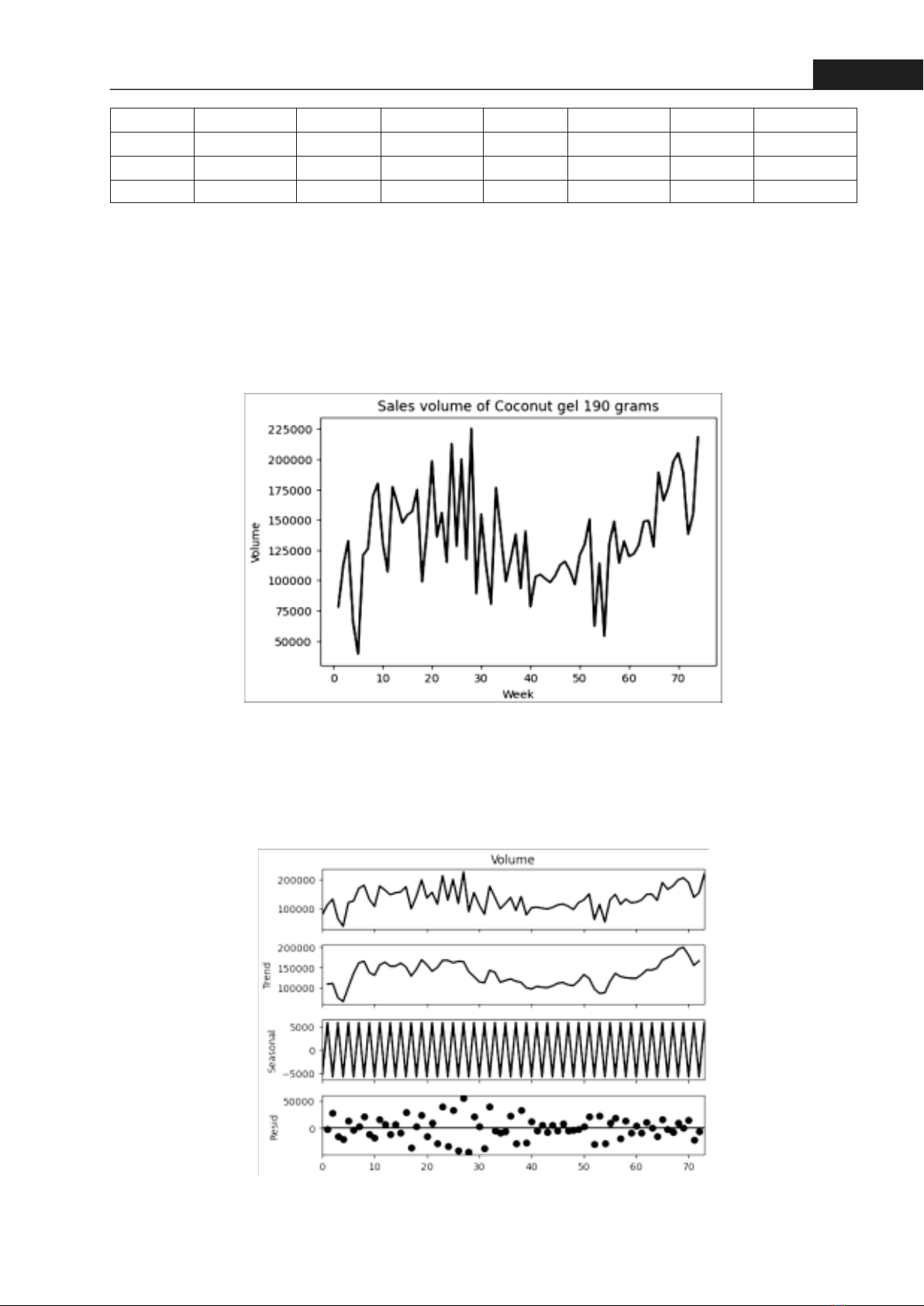
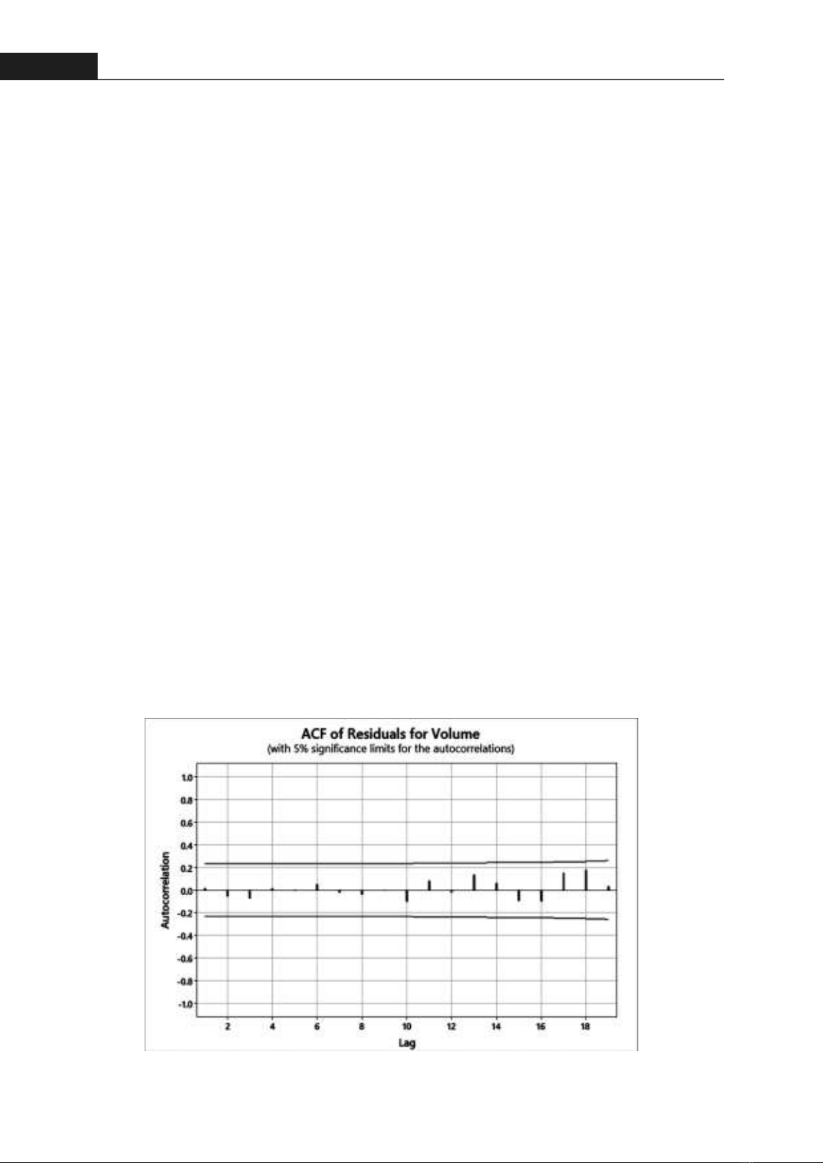
87Hong Bang Internaonal University Journal of ScienceISSN: 2615 - 9686 Hong Bang Internaonal University Journal of Science - Vol.5 - 12/2023: 85-92· Data analysisFrom the descripve analysis, the dataset exhibits the following characteriscs: The data ranges from 27,240 to 242,922, with an interquarle range of 109,062 to 155,590 and the presence of two outliers, detected using the 1.5 interquarle range rule [4]. The 1.5 interquarle range (IQR) rule is a stascal method to detect outliers in a dataset. It works by idenfying any data points that fall more than 1.5 mes the range from the ﬁrst quarle to the third quarle. Points which fall outside those limits usually indicate unusual ﬂuctuaons in demand. Therefore, it is necessary to replace these values using the 1.5 interquarle range rule [4]. The ﬁnal me series, aer treang the outliers, is shown in Figure 1.The me series has been decomposed in Figure 2. Time series decomposion has enabled us to separate the me series into three main components: trend, seasonality, and residual. From the trend component, it appears that there is a slight upward trend. Seasonality occurs with a period of two, as many retailers tend to import the company's products on a bi-monthly basis. Addionally, numerous irregular ﬂuctuaons in demand result in the variaon of residual data points.16 156886 35 99042 54 114276 73 154218 17 174881 36 117530 55 53964 74 218382 18 98908 37 138040 56 130188 19 142319 38 93319 57 148680 Figure 1. Time series plot aer replacing outliersFigure 2. Time series decomposion

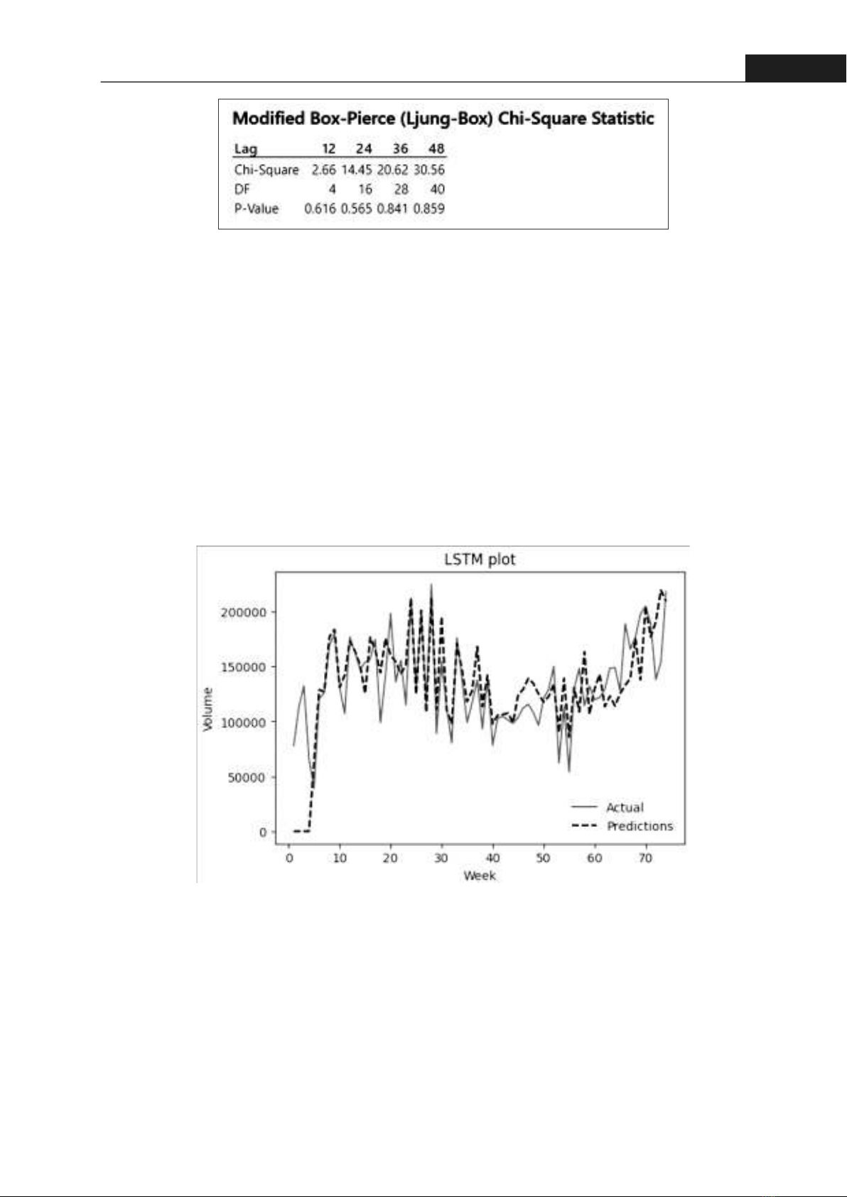
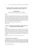
88Hong Bang Internaonal University Journal of ScienceISSN: 2615 - 9686Hong Bang Internaonal University Journal of Science - Vol.5 - 12/2023: 85-922.2. Model selecon and evaluaonThere are many methods that can be used to work well with the me series that has slight trend and seasonality with a strong irregular paer. ARIMA and LSTM models have been widely applied for me series forecasng tasks across domains. For instance, Williams et al [5] have developed seasonal ARIMA models to forecast traﬃc ﬂow. The models outperformed historical average benchmarks. Ediger et al [6] have applied ARIMA forecast primary energy demand in Turkey by fuel type. The models were able to accurately forecast primary energy demand for each fuel type one to ﬁve years ahead, with lower errors than alternave extrapolaon methods. On the other hand, LSTM also being applied in many research. Abbasimehr et al [7] have proposed an opmized LSTM model for product demand forecasng and compare performance against stascal methods. The opmized LSTM model signiﬁcantly outperforms the stascal methods across all forecast horizons, while the ARIMA and SARIMA performance degrades signiﬁcantly for longer horizon forecasts. In ﬁnance, Jiang et al [8] have developed a LSTM model to predict the stock market. The result states that the LSTM model outperformed the ARIMA model in forecasng stock prices in term of RMSE and MAPE metrics. However, some researches have provided the superiority of a combined LSTM-ARIMA model. G. Peter Zhang [9] has built a hybrid model combining ARIMA and neural networks for me series forecasng. The hybrid ARIMA-NN model signiﬁcantly outperforms both individual models across all forecast horizons on the two datasets. Similarly, Dave et al [10] have developed a hybrid ARIMA-LSTM model to forecast Indonesia's monthly export values and compare performance to individual models. The ARIMA-LSTM hybrid model provides the most accurate forecasts with lowest MAPE and RMSE scores across all horizons. It improves on individual models by 3-10%. By referring these researches, ARIMA, LSTM and a hybrid ARIMA-LSTM model is selected for this paper.2.2.1. ARIMA modelThe ARIMA model relies on three fundamental parameters-p, d, and q-each represenng a crucial aspect of the forecasng process. The variable “p” corresponds to the count of autoregressive terms (AR), indicang the reliance on past observaons for predicng future values while “d” signiﬁes the number of nonseasonal diﬀerences incorporated into the model, capturing the extent of data transformaon needed to achieve staonarity. Lastly, “q” denotes the quanty of lagged forecast errors (MA), reﬂecng the inﬂuence of past errors on the current predicon. By analyzing ACF and PACF plots, opmal parameters are chosen based on the informaon criteria (AIC), so the most suitable model is the ARIMA (4,0,4) [11].The ACF of residuals (Figure 3) shows that there is no lag value that fall outside the signiﬁcant limits. Furthermore, the p-value (Figure 4) for lag 12, 24, 36, and 48 all greater than 0.05. Therefore, there is not enough evidence to reject the null hypothesis of no autocorrelaon in the residuals, which can conclude that errors are random.Figure 3. The ACF plot of ARIMA's residuals

89Hong Bang Internaonal University Journal of ScienceISSN: 2615 - 9686 Hong Bang Internaonal University Journal of Science - Vol.5 - 12/2023: 85-922.2.2. LSTM modelThe LSTM model operates with disncve parameters that shape its architecture and inﬂuence its forecasng capabilies. Essenal elements such as the number of memory cells, layers, and other architectural features play a pivotal role in capturing intricate temporal dependencies within the sequenal data [12]. The LSTM model used in this paper is constructed with a sequenal architecture, featuring input layers with a shape of (4, 1). The core part of the model lies in the LSTM layer with 256 units and a recurrent dropout of 0.2, allowing it to capture temporal dependencies and paerns within the input data. The subsequent dense layers, each with 64 units and ReLU acvaon, add non-linearity to the model, enhancing its capacity to learn complex relaonships. The model is designed to predict a single output. During training, the mean squared error (MSE) is employed as the loss funcon, with the Adam opmizer ulizing a learning rate of 0.005. The model's performance is evaluated using mean absolute error as a metric. Training occurs over 200 epochs, with a batch size of 32. This architecture, through its LSTM structure and subsequent dense layers, is tailored to eﬀecvely capture and learn intricate paerns within sequenal data, making it a potent tool for forecasng and predicon tasks. 2.2.3. The hybrid ARIMA-LSTM modelIn general, both ARIMA and LSTM models have demonstrated success within their respecve linear or nonlinear domains, but these methods can't be applied to all scenarios. ARIMA's approximaon capabilies may fail to address complex nonlinear challenges, while LSTM, although suitable for handling both linear and nonlinear me series data, are hindered by prolonged training mes and a lack of clear parameter selecon guidelines [10]. Recognizing the limitaons of each model, a hybrid approach is employed, leveraging the individual strengths of ARIMA and neural networks. This hybrid model aims to enhance predicon accuracy by allowing the models to complement each other, overcoming their individual weaknesses. This strategy recognizes the composite nature of me series, considering a linear autocorrelaon Figure 4. The modiﬁed Box-Pierce Chi-Square stasc resultFigure 5. The LSTM model