
REGULAR ARTICLE
Evaluation of relevant information for optimal reflector modeling
through data assimilation procedures
Jean-Philippe Argaud
*
, Bertrand Bouriquet, Thomas Clerc, Flora Lucet-Sanchez, and Angélique Ponçot
EDF Recherche et développement, 1 avenue du Général de Gaulle, 92141 Clamart cedex, France
Received: 6 May 2015 / Received in final form: 28 July 2015 / Accepted: 6 November 2015
Published online: 16 December 2015
Abstract. The goal of this study is to look after the amount of information that is mandatory to get a relevant
parameters optimisation by data assimilation for physical models in neutronic diffusion calculations, and to
determine what is the best information to reach the optimum of accuracy at the cheapest cost. To evaluate the
quality of the optimisation, we study the covariance matrix that represents the accuracy of the optimised
parameter. This matrix is a classical output of the data assimilation procedure, and it is the main information
about accuracy and sensitivity of the parameter optimal determination. From these studies, we present some
results collected from the neutronic simulation of nuclear power plants. On the basis of the configuration studies,
it has been shown that with data assimilation we can determine a global strategy to optimise the quality of the
result with respect to the amount of information provided. The consequence of this is a cost reduction in terms of
measurement and/or computing time with respect to the basic approach.
1 Introduction
The modeling of the reflector part of a nuclear PWR core is
crucial to model the physical behaviour of the neutron
fluxes inside the core. However, this element is represented
by a parametrical model in the diffusion calculation code we
use. Thus, the determination of the reflector parameters is a
key point to obtain a good agreement with respect to
reference calculation such as transport one, used as pseudo-
observations. This can be done by optimisation of reflector
parameters with respect to reference values. This optimi-
sation needs to be done with care, avoiding in particular the
production of aberrant results by forcing the model to
match data that are not accurate enough or irrelevant. A
good way is to use data assimilation, to optimise by taking
into account the respective accuracy of core model and
reference values. This method allows to find a good
compromise between the information provided by the
model and the ones provided by a reference calculation.
Data assimilation techniques have already proven to be
efficient in such an exercise, as well as in field reconstruction
problems [1–5]. In particular, it has been shown that there is a
logarithmic-like progression of the quality of the reconstruc-
tion as a function of the number of instruments available.
Thus, there is an optimal amount of information that
provides suitable results without too many measurements.
The purpose of this work is to generalise and extend the
results, obtained previously on field reconstruction, for the
case of parameters optimisation. It is interesting to look for
the amount of information that is mandatory to get a
relevant parameters optimisation, and to determine what is
the best information to reach the optimum of accuracy at
the cheapest cost. This question is very important in an
industrial environment, as such knowledge helps to select
the most relevant reference values and then to reduce the
overall cost (measurement and/or computing cost) for
parameters determination.
In Section 2, we present a short review of data
assimilation concepts, giving the mathematical framework
of the method. Then we develop the specific equations that
are related to the purpose of information qualification.
Those developments highlight the opportunity given by
data assimilation to quantify the quality of the results. We
study the evolution of the trace of the so-called analysis
matrix Athat represents the accuracy of the optimised
parameter. This covariance matrix is a classical output of
the data assimilation procedure, and this is the main
information about accuracy and sensitivity of the optimal
parameter determination.
In Section 3, we present some results collected in the
field of neutronic simulation for nuclear power plants. Using
the neutronic diffusion code COCAGNE [6], we seek to
* e-mail: jean-philippe.argaud@edf.fr
EPJ Nuclear Sci. Technol. 1, 17 (2015)
©J.-P. Argaud et al., published by EDP Sciences, 2015
DOI: 10.1051/epjn/e2015-50022-3
Nuclear
Sciences
& Technologies
Available online at:
http://www.epj-n.org
This is an Open Access article distributed under the terms of the Creative Commons Attribution License (http://creativecommons.org/licenses/by/4.0),
which permits unrestricted use, distribution, and reproduction in any medium, provided the original work is properly cited.

optimise the reflector parameters that characterise the
neutronic reflector surrounding the whole reactive core in
the nuclear reactor. Those studies are done on several cases
which are required to be similar to the realistic configura-
tion of Pressurised Water Reactors (PWR) of type
900 MWe or 1300 MWe, respectively named PWR900
and PWR1300 hereafter.
Finally, we conclude with the best strategy, in order to
get the best result at the cheapest cost. This cost can be
either evaluated in terms of computing time or number of
reference measurements to provide.
2 Data assimilation and evaluation
of the quality
2.1 Data assimilation
Here we briefly introduce the key points of data assimila-
tion. More complete references on data assimilation can be
found in various publications [7–16]. However, data
assimilation is a wider domain and these techniques are,
for example, the keys of the meteorological operational
forecast. It is through advanced data assimilation methods
that the weather forecast has been drastically improved
during the last 30 years. Those techniques use all of the
available data, such as satellite measurements, as well as
sophisticated numerical models.
The ultimate goal of data assimilation methods is to
estimate the inaccessible true value of the system state, x
t
,
where the tindex stands for “true state”in the so-called
“control space”. The basic idea of most of data assimilation
methods is to combine information from an a priori
estimate on the state of the system (usually called x
b
, with
bfor “background”), and measurements (referenced as y
o
with ofor “observation”). The background is usually the
result of numerical simulations, but can also be derived
from any a priori knowledge. The result of the data
assimilation is called the analysis, denoted by x
a
, and it is
an estimation of the researched true state x
t
.
When adjusting parameters, the state xis used to
simulate the system using an operator named H, in order to
get output that can be compared to observations. This
operator embeds not only a physical equations simulator,
but also sampling or post-processing of the simulation in
order to get values that have the same nature as the
observation. For our data assimilation purpose, we use a
linearised form Hof the full non-linear operator H. The
inverse operation, to go from the observations space to the
background’s space, is formally given by the transpose H
T
of the linear operator H.
Two other ingredients are necessary. The first is the
covariance matrix of the observation errors, defined as
R= E[(y
o
–H(x
t
)).(y
o
–H(x
t
))
T
], where E[.] denotes the
mathematical expectation. It can be obtained from the
known errors on unbiased measurements, which means E
[y
o
–H(x
t
)] = 0. The second ingredient is the covariance
matrix of background errors, defined as B=E[(x
b
–x
t
).
(x
b
–x
t
)
T
]. It represents the error on the a priori state,
assuming it to be unbiased following the E[(x
b
–x
t
)] = 0 no
bias property. There are many ways to define this a priori
state and background error matrices. However, those
matrices are commonly the output of a model, the
evaluation of accuracy, or the result of expert knowledge.
It can be proved [7,8], within this formalism, that the
Best Unbiased Linear Estimator (BLUE, denoted as x
a
),
under the linear and static assumptions, is given by the
following equation:
xa¼xbþKy
oHx
b
;ð1Þ
where Kis the gain matrix:
K¼BHTHBHTþR
1
:ð2Þ
Equivalently, using the Sherman-Morrison-Woodbury
formula, we can write the Kmatrix in the following form
that we will exploit later:
K¼B1þHR1HT
1HTR1
:ð3Þ
Additionally, we can get the analysis error covariance
matrix A, characterising the x
a
analysis errors. This matrix
can be expressed from Kas:
A¼IKHðÞB;ð4Þ
where Iis the identity matrix.
If the probability distribution is Gaussian, solving
equation (1) is equivalent to minimize the following
function J(x), x
a
being the optimal solution:
JxðÞ¼ xxb
TB1xxb
þyoHxðÞðÞ
TR1yoHxðÞðÞ:ð5Þ
The minimization of this error (or cost function) is
known in data assimilation as the 3D-Var methodology
[10].
In the present case, we adjust the reflector parameter D
1
setting the diffusion characteristic of fast group neutrons in
diffusion equations, as described in details in reference [17].
2.2 Quality of data assimilation
One of the key points of data assimilation is that, as shown in
equation (4), we gain access to the Acovariance matrix. This
matrix characterises the quality of the obtained analysis. The
smaller the values in the matrix, the more “accurate”is the
final result. However, understanding the full matrix content
is tedious, so we choose to summarize it. For this purpose, we
look, classically, at the trace of the Amatrix, denoted as tr
(A), that is in fact the sum of all the analysis variances. The
smaller this value is overall, the better is the agreement.
According to our choice of the matrix trace as a quality
indicator, we take the Rand Bmatrices as diagonal in order
to get a posteriori information without adding too much a
priori information through terms outside the diagonal part of
the matrices. Moreover, this choice is the best if no extra
information is available on variances and covariances of
2 J.-P. Argaud et al.: EPJ Nuclear Sci. Technol. 1, 17 (2015)

errors. Thus, we consider diagonal matrices, with only one
parameter s
B
or s
R
, respectively, representing the overall
variance for each type of errors:
B¼sBIn
R¼sRIp
:ð6Þ
In these equations, the indices nand pstand for the size of
the space that is involved in control space (x
b
) and
observation space (y), respectively. With such a formulation,
we can write the gain matrix Kunder the following form:
K¼s2Inþs2HHT
1HT
;ð7Þ
with s2¼s2
B
s2
R
Then the matrix Ais:
A¼s2
BIns2Inþs2HHT
1HTH
:ð8Þ
Assuming that we only want to get the optimal value of
one parameter, as is often the case in optimal parameter
simple determination, we get HH
T
=h
2
, i.e. a scalar. Thus
we can write:
tr AðÞ¼ s2
B
1þs2h2:ð9Þ
This formulation has a very interesting asymptotic
behaviour. When the measurements are very inaccurate,
the result is only a function of s
B
, and when the background
is accurate the result depends on both the matrix product of
the observation operator HH
T
and on the accuracy of the
measurement.
In the case of one parameter to optimise pmeasurements,
the linear operator His a vector with pcomponents h
i
that
are respectively the linearisation of the ith component of the
operator Hfor the parameter laround the value lthat are
such that there is then one value of h
i
by measure with:
hi¼dHi
dl
lðÞ:ð10Þ
Under such conditions we can then write:
h2¼HHT¼X
p
i¼1
dH2
i
dl
lðÞ:ð11Þ
And then using equation (9) we can write:
tr AðÞ¼ s2
B
1þs2P
p
i¼1
dH2
i
dllðÞ
:ð12Þ
This formulation is very interesting as we see that the
more data we have, the higher is the value of h
2
, and the
higher is this value, the lower is the value of the trace of the
analysis.
There are two main ways to increase the value of h
2
. The
first one is to add more measurements in order to get a
higher value of p, assuming that we had a non-null value of
the derivative. This leads to the second option, which is the
increase of the sensitivity of the observation H
i
with respect
to the parameter l.
Moreover, the global structure of the function tr(A)as
(1 + x)
–1
shows that, as already expected, the improvement
of the quality is non-linear and saturating. Thus the
derivative is such that the first amount of information
provided has a huge impact in terms of decreasing the error
function. Then when the value of xincreases as we add
information, the function decreases more slowly (lower
value of the derivative), so a lot more information is
required to keep enhancing the quality.
In the present case, it is also worth noting that the
formulation in equation (10) is completely independent of
the experimental values themselves. It is only the setup and
the sensitivity to the parameter of the experiment that is
meaningful and that is given in the operator H.
3 Setup of the test and results
3.1 Setup of the problem for neutronic case
All the concepts and quality indicators that have been
presented in the previous section are now used in the case of
the neutronic problem, solved with the two energy groups
diffusion theory. The problem we plan to address is the
determination of an optimal parameter of the reflector D
1
in a
Lefebvre-Lebigot approach, where D
1
is the diffusion
coefficient of the fast group in the reflector. The aim is then
to know how many campaigns are necessary to determine the
best value of this parameter. To perform this task, we use the
core calculation code COCAGNE developed by EDF, with
the default parameters of several campaign that are
representative of the nuclear fleet, either of type PWR900
or type PWR1300. The campaigns have various lengths,
frequency of measurement and loading pattern setup to get a
rather realistic situation. We base our study on a set of 3
PWR900 campaigns, and on a set of 6 PWR1300 campaigns.
As already mentioned, there is no use of experimental or
measurement data in this study. We use equation (12) that
is dependent on Hbut not y(as in Eq. (1) and Eq. (5)), so it
is only the design of the campaign that matters through the
modeling of the Hobservation operator and its linearisation
H. In the considered campaign, for several values of burnup
(irregular to get closer to a real case), we consider the map
of activity in the core obtained through MFC (Mobile
Fission Chamber), as in the regular operation of operating
plants. The combination of the COCAGNE code and of the
mandatory post-processing to obtain the response of MFC
is the Hobservation operator. Its linearised approximation
His then obtained with finite differences around the
reference point.
3.2 Parameter determination on one campaign
We first study the impact of removing one or two
instruments on the final result through the value of
J.-P. Argaud et al.: EPJ Nuclear Sci. Technol. 1, 17 (2015) 3
tr(A), the trace of A. We make this study both on cases
similar to REP 900 and cases similar to PWR1300.
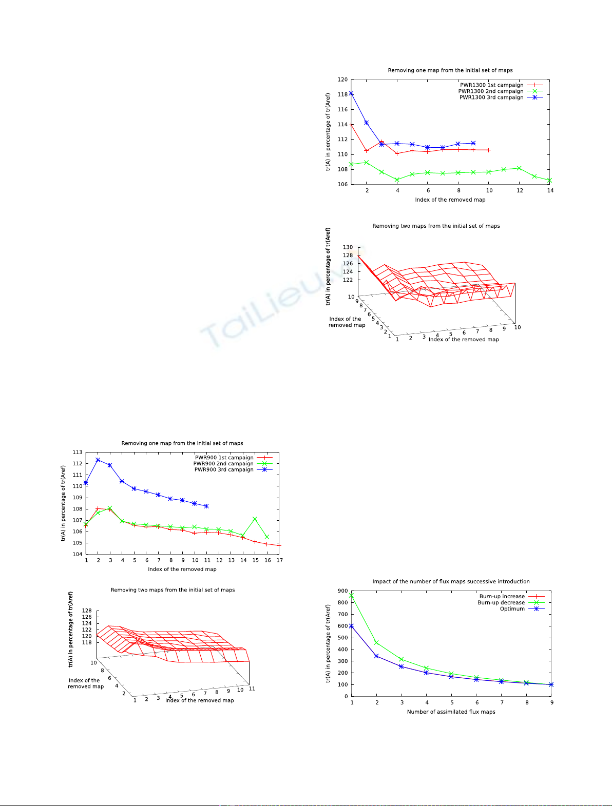
Figure 1 represents the evolution of the trace of A as we
remove, respectively, one or two maps from the collection of
available maps, for each studied campaign. The trace of A
is given as a percentage of the one calculated using all of the
available campaigns. When removing one measurement, we
can only decrease the quality of the analysis, leading to an
increase of the variance or the trace of A, and so all the
curves are above 100%. With such normalisation to the
limiting value, the curves can be compared between all of
the campaigns. In the top panel, we notice several points.
The first one, which is mathematically obvious but needs to
be recalled, is that the quality of the optimization decreases
when some maps are removed. This degradation is stronger
for the maps that are located at the beginning of the
campaign, and rather small for the maps located at the end.
Globally speaking, the decrease is steady between the
beginning and the end of the campaigns. For the bottom
panel of Figure 1, the conclusions are the same. The further
into the campaign a map is located, the smaller the effect of
removing this map.
In order to obtain a more global overview of the result,
we study the case of the PWR1300. In Figure 2, we plotted
the same information as in Figure 1, but for 3 cases among
the 6 of the PWR1300 set.
As in the case of the PWR900, it seems for PWR1300
that the maps at the beginning of the campaign are more
influential on the reflector result than those located at the
end. This result seems to be even clearer, as the slope of the
initial decrease looks to be sharper in Figure 2 than in
Figure 1. For the PWR900 campaigns, it is not straightforward to
conclude that the maps at the beginning of the campaign
are more interesting for data assimilation than the ones at
the end. To show more clearly that the maps at the
beginning are more important, we redo the work described
in Figure 3 in another way. For this purpose, we include in
the data assimilation more and more experimental flux
maps in two ways: the first consists of taking the map into
account following the increase of the burnup characteristic
(red curve) and the second consists of the opposite, that is
using the maps in decreasing order of burnup (green curve).
A third way is to look at the map that gives the best result,
and adding maps one by one in the same way (blue curve).
Fig. 1. Impact of removing one (top subplot) or two (bottom
subplot) maps on the quality of the parameter determination, as a
function of the index of the chosen map in 3 cases of PWR900
campaigns.
Fig. 2. Impact of removing one (top subplot) or two (bottom
subplot) maps on the quality of the parameter determination, as a
function of the index of the chosen map in 3 cases of PWR900
campaigns.
Fig. 3. Variation of the evolution of the trace of Aas a function of
the order of introduction of the flux maps in the data assimilation
process.
4 J.-P. Argaud et al.: EPJ Nuclear Sci. Technol. 1, 17 (2015)
Finally, when all of the information is added, all of the
curves reach the same point. With respect to what is plotted
in Figure 3, we noticed that a data assimilation procedure
taking into account the maps following increasing burnups
gives results that are very close to the optimal. On the
contrary, the assimilation procedure taking into account
the maps following decreasing burnups is not a good choice
when only a few maps are taken into account. Thus, even if
the curves that give the impact of removing one map are not
uniformly decreasing, we can still conclude that the maps
from the beginning of the campaign are more influential
than the maps at the end.
Thus, for data assimilation methods, some data are
more influential than others. The more the core is burnt, the
less the map seems to be influential in decreasing the trace
of A. The burning of the core tends to make the flux map
spatially more homogeneous (“flat”). As the D
1
reflector
parameter governs mainly the global curvature of the flux
inside the reactive core, if it is determined on a quasi-fully-
burnt core with very flat flux map, the resulting D
1
will be
very insensitive to the burnup.
It is then possible to determine a strategy in using this
framework to get optimal results at the lowest cost.
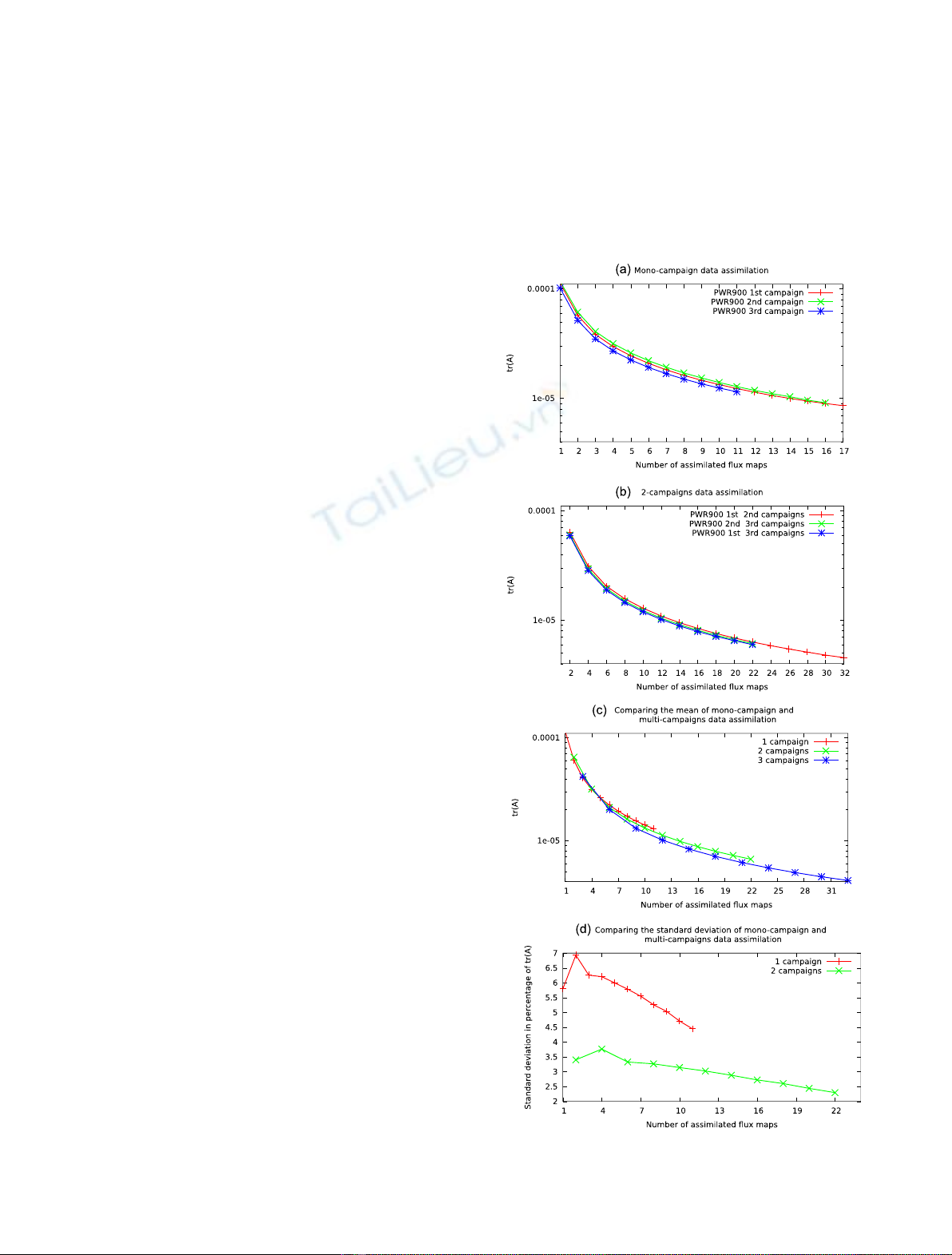
3.3 Parameter determination on several campaigns
As a global multi-campaigns strategy of optimisation can
be determined, we go to the next step. We compare the
trace of the matrix calculated from multiple campaigns to
that coming only from one campaign. We build multi-
campaigns cases in the following way. Assuming that we
dispose of the flux maps coming from 3 campaigns, we solve
a data assimilation problem with the first map of each
campaign. Thus we obtain a first analysis and value of
tr(A). Then, we use in addition the second map of each of
the three campaigns, and we obtain a new analysis for a
total of six maps, and so on.
To make a good comparison, we also show the evolution
of tr(A) for data assimilation with only one campaign. For
those curves, the first point is obtained using the first
available map then the second using the two first maps, and
so on.
In order to make a comparison between the multi-
campaigns data assimilation, we calculate statistical
indicators (mean and standard deviation) for each kind
of multi-campaigns data assimilation (use of 2 campaigns, 3
campaigns . . . ) on all the possible combinations. For
example, for the data assimilation of 3 campaigns over a set
of 6, like in PWR1300, there are 20 possible combinations.
Those statistical indicators are given in all the coming
figures. It is worth pointing out that the standard deviation
does not correspond to the standard deviation on the
analysis (which is here directly tr(A) but to the standard
deviation of tr(A). Here, we are studying the variability of
the indicator tr(A) as a function of the chosen set of
campaigns.
For the PWR900, we have 3 campaigns with associated
calculations of flux maps. In Figures 4a–4c, we present the
evaluation of the trace of A as a function of the total
number of maps assimilated, respectively for 3 scenarios of
data assimilation: mono-campaign data assimilation (3
cases), 2-campaign data assimilation (3 cases), and 3-
campaign data assimilation (1 case). The data for mono-
campaign and 2-campaign are a mean value on the different
results for each scenario. Figure 4d presents the compared
evolution of the standard deviation for the mono-campaign
and 2-campaigns cases.
Fig. 4. Evolution of the trace of Aas a function of the number of
assimilated flux maps for the PWR900.
J.-P. Argaud et al.: EPJ Nuclear Sci. Technol. 1, 17 (2015) 5


![Đề ôn tập cuối kỳ môn Kỹ thuật nhiệt - Nhiệt động học [mới nhất]](https://cdn.tailieu.vn/images/document/thumbnail/2026/20260310/hoaphuong0906/135x160/60681773197823.jpg)

![Bài giảng thang máy và thang cuốn: Tổng hợp kiến thức [chuẩn nhất]](https://cdn.tailieu.vn/images/document/thumbnail/2026/20260310/hoaphuong0906/135x160/41471773283876.jpg)
