Tối ưu bài toán Job Shop Scheduling: Lịch trình tổng thể dựa trên thuật toán di truyền cải tiến

ISSN 1859-1531 - THE UNIVERSITY OF DANANG - JOURNAL OF SCIENCE AND TECHNOLOGY, VOL. 22, NO. 12, 2024 7

AN INNOVATIVE GENETIC ALGORITHM-BASED MASTER SCHEDULE TO

OPTIMIZE JOB SHOP SCHEDULING PROBLEM

Thi Phuong Quyen Nguyen*, Thi Hoa Thuong Le

The University of Danang - University of Science and Technology, Vietnam

*Corresponding author: ntpquyen@dut.udn.vn

(Received: September 27, 2024; Revised: October 29, 2024; Accepted: November 01, 2024)

DOI: 10.31130/ud-jst.2024.422E

Abstract - The rapid development of manufacturing sectors in the

contemporary Industry 4.0 era has prompted enterprises to adopt

increasingly systematic, streamlined, and efficient organizational

structures. In this scenario, production scheduling has arisen as an

essential function that contributes to the effective allocation of

organizational resources in the production process, while

shortening production time and satisfying customer deadlines.

Consequently, the objective of this study is to develop an advanced

method to optimize the production scheduling problem.

Accordingly, this study proposes an innovative genetic algorithm-

based master schedule (GA-MS) focused on minimizing makespan.

The proposed method is implemented in various benchmark

datasets on job shop scheduling problems. Compared with some

benchmark methods such as priority rules-based approaches,

branch and bound algorithm (B&B), and shifting bottleneck

algorithm (SB), the proposed GA-MS shows an outstanding

performance concerning the tested datasets. Its application in

practical manufacturing factories is highly recommended.

Key words – Job shop scheduling problem; genetic algorithm;

master schedule.

1. Introduction

In today's competitive environment, production

scheduling plays a very important role in the sustainability

of enterprises within the marketplace. To fulfill customer

demands, such as timely delivery, organizations must

develop a precise strategy, adeptly allocate, and utilize

available resources effectively and reasonably. If a firm

underestimates the importance of production scheduling, it

may face many difficulties in its operations, resulting in

resource inefficiency, reduced productivity, and substantial

cost increases [1].

There are many types of production scheduling models

such as single machine scheduling model, flow shop, job

shop scheduling model, open shop, and so on. However,

the job shop scheduling problem (JSSP) is the most popular

one in practical issues. JSSP is a production or service

model in which each job has a separate route through

different machines or equipment. In the JSSP model, there

is always a conflict over resources such as human resources

and equipment. Thus, JSSP is a difficult problem among

all types of scheduling problems [2].

The JSSP in manufacturing industries is characterized

by multifunctional machinery and equipment that produces

multiple products with a wide range of features processed

on a variety of machines, each of which can process a large

number of details [3]. For example, printed circuit boards

in the semiconductor industry are often produced in the

form of job shops; orders are usually a certain batch of

products, carried out through a given route with specific

execution times.

The JSSP is classified as the NP-hard (Non-

Polynominal-hard) problem and cannot be solved like

normal linear programming problems [4]. Various meta-

heuristics approaches have been proposed to solve JSSP,

such as genetic algorithms (GA) [5, 6], evolutionary

algorithms [7, 8], ant colony optimization [9], and particle

swarm optimization (PSO) [10]. Among these meta-

heuristics approaches, GA is the most popular one for

solving optimization problems [11].

Thus, this study proposes an innovative genetic

algorithm-based master schedule (denoted as GA-MS) to

optimize the JSSP. A master schedule (MS) is a matrix that

shows the sequence of jobs processed in each machine.

Each MS is coded as a chromosome. An innovative method

is developed to generate numerous MS for the initialization

of GA procedure in which each MS can avoid infeasible

solutions due to the job’s sequence constraint. Thereafter,

the genetic operation is implemented to determine the

optimal solution to minimize makespan for JSSP.

2. Related works

2.1. Overview of JSSP

Table 1. Notations of JSSP

Number of jobs

Number of machines

Index of machines, i=1, 2,…, m

Index of jobs, j=1, 2,…, n

pij

Processing time of job j on machine i

xij

Starting time of job j on machine i

Release date/ Ready date of job j

Due date of job j

Completion time of job j

𝐶𝑚𝑎𝑥

Make-span 𝐶𝑚𝑎𝑥= max{Cj: j = 1, 2, …, n}

Flow time job j

Lateness (Lj = Cj – dj)

Tardiness Tj = max (0, Lj).

The classical JSSP is identified in manufacturing in

which n different jobs/products are to be scheduled on m

different machines, subject to two main sets of constraints

which are the precedence constraints and the conflict

constraints. Each job has a different sequential operation.

The processing time of each job on machines is known,

consistent, and independent of the schedules on machines.

8 Thi Phuong Quyen Nguyen, Thi Hoa Thuong Le

The objective of JSP is to sequence jobs on machines and

specify the starting time and ending time of each job to

minimize certain performance. In this case, the objective

function is to minimize makespan. Some notations of JSSP

are listed in Table 1.

The problem can be modeled as follows:

Objective function

Min 𝐶𝑚𝑎𝑥 (1)

S.t.

∑𝑌𝑖𝑗𝑗′= 1

𝑛

𝑗′=1

𝑗′≠𝑗

(2)

∑𝑌𝑖𝑗𝑗′= 1

𝑛

𝑗=1

𝑗≠𝑗′

(3)

xij+ pij ≤ xi’j (4)

xij+ pij ≤ xij’ + M(1 − Yijj’) (5)

xij’+ pij’ ≤ xij + MYijj’ (6)

xij≥ rj≥ 0 (7)

Cj = xlj + plj (8)

Eq. (1) is used for the objective function that is

minimizing make-span 𝐶𝑚𝑎𝑥= max{Cj: j = 1, 2, …, n}.

Eq. (2) indicates that on each machine i, when a job

completes its processing, only one job in the set of

available jobs is selected for processing. Eq. (3) means an

operation of a job should follow only one processor. Eq.

(4) is used for the precedence constraints. The precedence

constraints ensure that each operation of a certain job is

processed sequentially. Eq. (5) and (6) present the conflict

constraints where M is a constant that is assumed to be a

big number. The conflict constraints guarantee that each

machine processes only one job at a time. Eq. (7) is to make

certain that any job cannot start before its ready time. Eq.

(8) is a formulation to identify the completion time of each

job on each machine. Variable “l” in Eq. (8) is the last

machine that product j is processed on. Eq. (9) explains the

binary variable 𝑌

𝑖𝑗𝑗’. 𝑌

𝑖𝑗𝑗’ = 1 if job j is produced before job

j’ on machine i. Unless, 𝑌

𝑖𝑗𝑗’ will get a value of 0.

2.2. Priority rules-based methods for scheduling problems

This section introduces some methods to solve the

scheduling problems based on the priority rules. A priority

rule is a type of policy that determines a specific

sequencing choice for each time a machine idles. A priority

rule is a type of policy that determines a specific

sequencing choice for each time a machine idles [12].

Some priority rule-based methods can be listed as follows:

(1) Earliest Due Date (EDD): The job with the earliest

due date is selected to be executed first in which the goal

is to minimize maximum lateness.

(2) Longest Processing Time (LPT): the sequence of

jobs depends on its processing time. The job with the

largest processing time will be scheduled first. This rule is

usually applied in parallel machine models to balance the

workload across machines.

(3) Weight Shortest Processing Time (WSPT): The job

with the largest ratio (wj/pj) is done first. This rule aims to

minimize the total weighted completion time ∑𝑤𝑗𝐶𝑗. When

all weights are equal, the WSPT rule becomes the SPT rule.

(4) Minimum Slack (MS): When a machine is idle at

time t, the remaining slack time of each job at that time t is

defined as:

Slack = (dj – pj – t) (10)

Slack will be negative for late jobs, zero for on-time

jobs, and positive for early jobs.

(5) Shortest Set-up Time (SST): This rule selects the job

that has the smallest set-up time to implement first.

(6) Least Flexible Job (LFJ): This rule selects the job

with the least flexibility to process (the least flexible job

can only be executed on a certain number of machines or

processed by the fewest number of machines). This rule is

suitable for the heterogeneous parallel machine model.

(7) Critical Path (CP): Select the job on the critical

path to perform first, suitable for jobs with precedence

constraints.

(8) Largest Number of Successors (LNS): Choose the

job with the longest list of following jobs to do first.

2.3. Heuristic methods for JSSP

Branch and Bound (B&B): The B&B [13] constitutes

an enumeration technique whereby all conceivable job

sequences are cataloged within a hierarchical structure.

Subsequently, the array of scheduling tables is sequentially

eliminated by demonstrating that the target values

associated with all schedules exceed a predetermined lower

bound. This lower bound is defined as being greater than

or equal to the target value of a previously attained

schedule. The B&B is extensively employed to ascertain

an optimal solution to the scheduling problem.

Nonetheless, it is characterized by significant time

consumption, as the number of nodes is often very large.

Genetic Algorithm (GA): GA [5, 6] aims to develop

solutions that outperform their parents by utilizing diverse

methodologies. GA begins with the initialization step, which

simultaneously creates a population with many solutions.

The best solutions are then selected from the generated

alternatives. Thereafter, genetic operators, including

crossover and mutation processes, are used for these selected

individuals to generate offspring under the principle of an

evolutionary process, i.e., the next generation is always

better than the previous generation. This iterative procedure

persists until an optimal solution is attained.

Particle Swarm Optimization Algorithm (PSO): PSO

[10] is an algorithm designed to address optimization

problems on an intelligent population model or intelligent

swarm. PSO is a straightforward but efficient technique for

optimizing continuous nonlinear objective functions. It has

been effectively applied to solve numerous function

extremum problems as well as multi-objective problems.

This study uses GA-based MS to optimize the JSSP. GA is

selected among other heuristic methods due to its effectiveness

has been proven in many optimization problems [5, 6].

Yijj’ =

0 otherwise

1 if job j is before job j’ on machine i

(9)

ISSN 1859-1531 - THE UNIVERSITY OF DANANG - JOURNAL OF SCIENCE AND TECHNOLOGY, VOL. 22, NO. 12, 2024 9

3. Proposed GA-MS for JSSP

The idea for the proposed GA-MS to solve the JSSP is

developed based on the MS. Each MS is a solution for the

JSSP, i.e., a sequence of jobs to be processed on machines.

The procedure of the proposed GA-MS begins with the

initialization process based on designing and generating the

MS. Then, the proposed GA-MS will follow the general

procedure of genetic operation until obtain optimal solution.

The details will be presented in the following subsections.

3.1. Master Schedule

MS is a combination of schedules for each job/product

on each machine in the production process. Note that the

processing time is known, consistent, and independent of

the schedules on machines. Therefore, the result of the

JSSP is to know the schedules for jobs/products on all

machines, which is called the MS. However, each product

has to follow its processing sequence which is known as

precedence constraint. Thus, it is necessary to consider

how one machine's schedule will affect the schedules of the

remaining machines when generating a feasible MS.

An example is given to illustrate how to generate an

MS. Given a JSSP with 3 jobs and 2 machines, the

sequence of performing each job on the machines is shown

in Table 2. The number in a row in Table 1 represents the

order of machines that process jobs. For instance, Job 1 (J1)

is processed on M1 first, then goes to M2. The sequence of

Job 2 (J2) is on M2 first then moves to M1.

Table 2. Sequence matrix in JSSP

Sequence

Machine

Job

The processing time of a job on one machine is shown

in Table 3. It is identified based on the job row and machine

column. For instance, the processing time of J1 on M1 is

14; the processing time of J2 on M1 is 6.

Table 3. Sequence matrix in JSSP

Processing Time

Machine

Job

Table 4 illustrates an MS. In the MS matrix, the

schedule on one machine is represented in an equivalent

column of the machine. For instance, the sequence of jobs

processed on machine M1 is J2-J1-J3, and on machine M2

is J1-J2-J3.

Table 4. An illustration of an MS

Master Schedule

Machine

Job

Referencing the MS in Table 3, the solution is infeasible

because the schedule conflicts with the processing sequence

in Table 1. For instance, M1 cannot process J2 first since it

has to wait for the completion of J2 on M2. However,

according to the MS, J2 cannot be processed on M2 because

M2 has to process J1 first. Similarly, J1 cannot be processed

on M2 due to the processing sequence and J1 needs to go to

M1 first. As a result, the schedule is blocked.

Thus, this study develops a method to generate an MS

that can avoid infeasible solutions. The concept to generate

the feasible MS is to select one machine as the “Main

Machine”. Schedules on other machines are based on the

schedule on the Main Machine and the sequence matrix.

For the above example, suppose that we select M1 as

the Main Machine, and assign the schedule on M1 as Table

4. Then, we will generate the schedule on M2 as follows:

Step 1: Consider the column M2 of the sequence

matrix, only J2 is available to be processed in M2, hence

assign J2 to M2. The result is illustrated in Table 5.

Table 5. An illustration to generate a feasible MS

Sequence

Machine

Master

Schedule

Machine

Job

Step 2: Due to Step 1, J2 is assigned to be the first in

M2; hence J2 can be processed on M2, then on M1. When

M1 completes J2, it will continue with J1 without violating

the J1 processing sequence. After J1 is completed, J3 is

processed on M1 as scheduled on M1 is J2-J1-J3. The

current schedule is presented in Table 6. In the sequence

matrix, “0” means already finished jobs while “1” means

available jobs to be processed.

Table 6. An illustration to generate a feasible MS

Sequence

Machine

Master

Schedule

Machine

Job

Step 3: Both J1 and J3 are available, we assign them in

M2 based on the available time rule, which is the sooner

the product is available, the higher the probability to be

assigned before the others. This rule can enhance the

diversity of solutions to large-scale problems. The

schedule shown in Table 7 is a feasible MS.

Table 7. An illustration to generate a feasible MS

Sequence

Machine

Master

Schedule

Machine

Job

3.2. Proposed GA-based MS

3.2.1. Chromosome representation

A chromosome is coded as a feasible MS. According to

Section 3.1, a feasible MS is a matrix type where the

10 Thi Phuong Quyen Nguyen, Thi Hoa Thuong Le

schedule on each machine is shown in the path

representation. For instance, the sequence in M1 in Table

7 is J2→ J1→ J3. Because of precedence constraints, each

job will follow its processing sequence. It leads to the

schedules in the path representations that have different

length sizes. Table 8 illustrates this case.

Table 8. An MS with different length sizes in each machine

Machine

Job

Thus, a feasible MS should be coded in the matrix

representation with the length consistently. From Table 8,

an MS with the same is transformed and shown in Table 9.

The number in Table 9 shows the order of jobs that are

processed in each machine. For instance, J1 is processed in

M1 first, thus the cell M1J1=1. J1 does not go to M2, so

the cell M2J1=0. Similarly, J1 is executed in M1 in the 3rd

order. Thus, the cell M3J1 gets a value of 3. This way is

used to transform all jobs in Table 8 to Table 9.

Table 9. An MS in the matrix representation

Machine

Job

3.2.2. Initialization

Each MS represents a chromosome. To generate a

population-based MS, the study designs to code a number

that is equivalent to a schedule on each machine. Following

the process to generate an MS, after choosing a Main

Machine, the sequence of jobs processed on the Main

Machine is determined. The number of possible schedules

also has to be defined on the Main Machine. For example,

if we have a job list including n jobs that will be processed

on the Main Machine; it means we will have n factorial

permutation schedules of n jobs. Each possible schedule is

equivalent to one unique value. Based on the population

situation of each iteration, each individual (chromosome)

is represented by one value. Converting the value of an

individual into one unique schedule on the Main Machine

will be followed in these steps.

Step 1

Order the job list including n jobs

Pick up Value

Calculate Order = roundup (Value/(n-1)!)

Select a job on the list as the first order at machine.

Step 2

Update Job List: (n-1) jobs

Order the remaining job list

Calculate Update Value = previous Value - (n-1)!

*(previous Order-1)

Calculate Update Order = roundup (Update

Value/((n-1)-1)!)

Select a job on the list as the second order at machine

Step 3: Repeat step 2 until the final job on the list

Table 10 shows the possible schedule of 4 jobs on the

Main Machine. The schedules of these jobs in other

machines are determined based on the process of

generating an MS. Then, all possible MSs are used for the

initial population.

Table 10. Schedule on Main Machine with n=4

Value

Schedule

Value

Schedule

1 – 2 – 3 – 4

3 – 1 – 2 – 4

1 – 2 – 4 – 3

3 – 1 – 4 – 2

1 – 3 – 2 – 4

3 – 2 – 1 – 4

1 – 3 – 4 – 2

3 – 2 – 4 – 1

1 – 4 – 2 – 3

3 – 4 – 1 – 2

1 – 4 – 3 – 2

3 – 4 – 2 – 1

2 – 1 – 3 – 4

4 – 1 – 2 – 3

2 – 1 – 4 – 3

4 – 1 – 3 – 2

2 – 3 – 1 – 4

4 – 2 – 1 – 3

2 – 3 – 4 – 1

4 – 2 – 3 – 1

2 – 4 – 1 – 3

4 – 3 – 1 – 2

2 – 4 – 3 – 1

4 – 3 – 2 – 1

3.2.3. Evaluation of Fitness Value

The study considers minimizing the value of makespan.

Makespan is the total time required to complete a set of

jobs from the beginning of the first job to the end of the

final job.

Make-span 𝐶𝑚𝑎𝑥= max{Cj: j = 1, 2, …,n} (10)

3.2.4. Genetic operation

The genetic operation includes the selection, crossover,

and mutation process. The proposed GA-MS employs the

Roulette Wheel method for the selection process to choose

the parent chromosomes for producing the next generation.

Regarding the crossover process, the traditional one-point

crossover is utilized in which a random position in two

selected chromosomes is picked up to perform crossover.

Similarly, the mutation process is performed on a schedule

of the Main Machine by randomly selecting two jobs and

swapping two jobs at selected locations.

The offspring are produced after the genetic operation.

The process is repeated to evaluate the fitness values of the

offspring and continue with the genetic operation to

reproduce the next generation. This process is repeated

until the stopping criteria are met.

Some advances are designed in the proposed GA-MS.

First, parameters are adjusted to encourage diversity during

early iterations, thereby enhancing the exploration of the

global optimum. Additionally, to improve exploitation to

the local optimum, 10% of the population is replaced by

very good solutions when the total number of iterations

exceeds 90% or the best solution consistently persists for

40% of the total iterations. This strategy enables the

population to conduct a dense search for the very best

answers. To cut down on running time, the program is

designed to self-terminate if the optimal solution remains

unchanged after 50% of the total iterations.

ISSN 1859-1531 - THE UNIVERSITY OF DANANG - JOURNAL OF SCIENCE AND TECHNOLOGY, VOL. 22, NO. 12, 2024 11

4. Experimental Result

4.1. Parameter setting

To implement the proposed GA-MS, some parameters

need to be set up such as the number of iterations (ItNum),

population size (Popsize), probability of crossover:

(Prob_CO), probability of Mutation (Prob_Mut). The

values of ItNum and Popsize are chosen according to the

experimental results of some previous research. The

crossover rate Prob_CO is from 0.8 to 1.0. A high

crossover rate is selected to lead to premature convergence.

The mutation rate Prob_Mut is usually from 0.005 to 0.1.

In this case, the high mutation rate is selected to enhance

diversity. Finally, we experiment with multi-trials and

determine the parameter for the proposed GA-MS as

follows: ItNum = 200, Popsize = 100, Prob_CO = 0.8, and

Prob_Mut = 0.1

4.2. Dataset

Ten tested datasets collected from OR-Library

(http://people.brunel.ac.uk/~mastjjb/jeb/orlib/jobshopinfo.

html) are employed to implement and evaluate the

performance of the proposed GA-MS. These datasets are

usually used as the benchmarks for JSSP. The tested

datasets can be classified into three types: 1) small-scale

problems with n, m  4; 2) medium-scale problems with

4 < 𝑛, 𝑚  10; 3) large-scale problems with 𝑛, 𝑚 > 10.

There are three small-scale datasets, four medium-scale

datasets, and three large-scale datasets.

4.3. Result analysis

To evaluate the effectiveness of the proposed GA-MS,

some benchmark algorithms are also used to compare its

performance. This study selects the EDD rule since it is the

most popular one among other priority rule-based methods.

Besides, B&B and shifting bottleneck (SB) methods are

also chosen as benchmark algorithms due to their simple

but straightforward and efficient in solving JSSP.

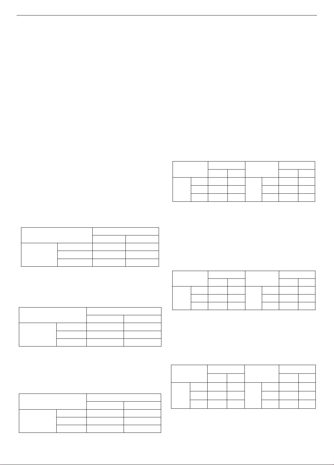
Table 11. The experimental result

Dataset

EDD

B&B

GA-MS

461

262

273

215

138

150

131

142

110

118

104

837

790

798

736

1286

1022

983

1854

1682

1676

1392

2717

2523

2598

2152

The proposed GA-MS is implemented 20 times on each

tested dataset and its average result is obtained. Table 11

shows the results of the proposed GA-MS with the three

benchmark algorithms. The value in Table 11 is the

makespan in which the smaller makespan is the better

algorithm. The makespan was computed for each method

based on Eq. (10) with its notation presented in Table 1.

The result in Table 11 exhibits that the best makespan

values vary based on the scale of problems. For small-scale

problems, which are shown by the result of datasets 1 to 3,

it is obvious that the GA-MS outperforms the other

benchmarks since it achieves two best makespans on

datasets 2 and 3. The B&B and SB algorithms rank the

second order with the best makespan on dataset 1. EDD

cannot obtain any best makespan on small-scale datasets.

However, there is not a big difference between these

algorithms in terms of makespan in these datasets. For

example, the best makespan of dataset 2 provided by GA-

MS algorithms is 26 while the worst makespan obtained by

EDD is 35. The gap in makespan between GA-MS and

B&B is also small with only 6.

Figure 1. The comparison results on different datasets

Regarding the medium-scale problems from datasets

4 to 7, the proposed GA-MS is still the best one since it

obtains the best performance on 3 datasets. Especially,

the difference in makespan between the proposed GA-MS

and EDD method is relatively large. This illustrates the

effectiveness of the proposed GA-MS when the scale of

problems increases. The result is similar to the large-scale

problems shown in datasets 8 to 10. It is noted that as

problem sizes rise, the makespan gaps between the

suggested GA-MS and B&B and GA-MS and SB also

widen. Generally, heuristic methods such as EDD, B&B,

and SB are ineffective for large and complicated

problems. The proposed GA-MS can find the optimal

solutions for these JSSPs quickly and efficiently. The

computational time to implement the proposed GA-MS is

also promising. It only takes from few seconds for the

small-scale dataset to less than 5 minutes for the large-

An innovative genetic algorithm-based master schedule to optimize job shop scheduling problem

Chủ đề:

Tài liệu liên quan

Tài liêu mới

AI tóm tắt

Giới thiệu tài liệu

Đối tượng sử dụng

Từ khoá chính

Nội dung tóm tắt

Hỗ trợ

Phương thức thanh toán

Theo dõi chúng tôi