Master's thesis of Engineering: Detailed analysis of the relationship between geometry and airflow in older Chinese adult male nasal cavities

Detailed Analysis of the Relationship between Geometry and Airﬂow in Older Chinese Adult Male Nasal Cavities

A thesis submitted in fulﬁlment of the requirements for the degree of Masters by research

Sean Dermott Read

School of Aerospace Mechanical and Manufacturing Engineering

College of Science Engineering and Health

RMIT University

October 2016

Declaration

I certify that except where due acknowledgement has been made, the work is that of the author alone; the work has not been submitted previously, in whole or in part, to qualify for any other academic award; the content of the thesis is the result of work which has been carried out since the oﬃcial commencement date of the approved research program; any editorial work, paid or unpaid, carried out by a third party is acknowledged; and, ethics procedures and guidelines have been followed

Sean Dermott Read

28th October 2016

Acknowledgements

I want to thank my supervisors, Dr Kiao Inthavong and Professor Jiyuan Tu, my colleagues in the CFD group, my family and my partner Tao Yao.

III

Abstract 1

1 Introduction 3

3 1.1 Background . . . . . . . . . . . . . . . . . . . . . . . . . . . .

5 1.2 Literature review . . . . . . . . . . . . . . . . . . . . . . . . .

5 1.2.1 Nasal cavity anatomy . . . . . . . . . . . . . . . . . . .

6 1.2.2 Geriatric rhinology . . . . . . . . . . . . . . . . . . . .

7 1.2.3 Experimental studies in rhinology . . . . . . . . . . . .

8 1.2.4 Computational studies . . . . . . . . . . . . . . . . . .

1.2.5 Geometric variations . . . . . . . . . . . . . . . . . . . 11

1.2.6 Fluid dynamics . . . . . . . . . . . . . . . . . . . . . . 12

1.2.7 Demographic studies . . . . . . . . . . . . . . . . . . . 17

1.3 Summary . . . . . . . . . . . . . . . . . . . . . . . . . . . . . 17

1.4 Literature gap . . . . . . . . . . . . . . . . . . . . . . . . . . . 18

1.5 Research questions and objectives . . . . . . . . . . . . . . . . 19

1.6 Research overview . . . . . . . . . . . . . . . . . . . . . . . . . 20

2 Model reconstruction and meshing 21

2.1 Introducton . . . . . . . . . . . . . . . . . . . . . . . . . . . . 21

2.2 Geometry . . . . . . . . . . . . . . . . . . . . . . . . . . . . . 22

2.2.1 Introduction . . . . . . . . . . . . . . . . . . . . . . . . 22

2.2.2 Non-invasive medical imaging . . . . . . . . . . . . . . 22

2.2.3 Image segmentation . . . . . . . . . . . . . . . . . . . . 23

2.2.4 Preparation of model for meshing . . . . . . . . . . . . 25

2.2.5 Summary . . . . . . . . . . . . . . . . . . . . . . . . . 25

2.3 Meshing . . . . . . . . . . . . . . . . . . . . . . . . . . . . . . 27

2.3.1 Introduction . . . . . . . . . . . . . . . . . . . . . . . . 27

2.3.2 Mesh types . . . . . . . . . . . . . . . . . . . . . . . . 27

2.3.3 Meshing algorithms . . . . . . . . . . . . . . . . . . . . 30

2.3.4 Quality . . . . . . . . . . . . . . . . . . . . . . . . . . 30

2.3.5 Mesh independence . . . . . . . . . . . . . . . . . . . . 31

2.3.6 Meshing of the nasal cavity . . . . . . . . . . . . . . . 33

3 CFD fundamentals 37

3.1 Introduction . . . . . . . . . . . . . . . . . . . . . . . . . . . . 37

3.2 Fluid Dynamics . . . . . . . . . . . . . . . . . . . . . . . . . . 37

3.2.1 Mass conservation . . . . . . . . . . . . . . . . . . . . . 38

3.2.2 Momentum conservation . . . . . . . . . . . . . . . . . 40

3.2.3 Energy Conservation . . . . . . . . . . . . . . . . . . . 42

3.3 Humidity . . . . . . . . . . . . . . . . . . . . . . . . . . . . . 43

3.4 Solving the governing equations . . . . . . . . . . . . . . . . . 45

3.4.1 Discretisation . . . . . . . . . . . . . . . . . . . . . . . 45

3.4.2 Numerical Solution . . . . . . . . . . . . . . . . . . . . 46

3.5 Setup and solution of nasal cavity models used in this thesis . 47

4 Results 49

4.1 Introduction . . . . . . . . . . . . . . . . . . . . . . . . . . . . 49

4.2 Wall shear stress and velocity . . . . . . . . . . . . . . . . . . 49

4.3 Geometry Variations . . . . . . . . . . . . . . . . . . . . . . . 58

4.4 Pressure drop . . . . . . . . . . . . . . . . . . . . . . . . . . . 66

4.5 Heat and vapour transfer . . . . . . . . . . . . . . . . . . . . . 69

71 5 Discussion

5.1 Conclusions . . . . . . . . . . . . . . . . . . . . . . . . . . . . 77

5.2 Future works . . . . . . . . . . . . . . . . . . . . . . . . . . . 78

VII

List of Figures

1.1 Cross-section through the middle of the nasal cavity Showing the olfactory region (upper shaded area). NV, nasal vestibule; IT, inferior turbinate and oriﬁce of the nasolacrimal duct; MT, middle turbinate and oriﬁces of frontal sinus, anterior eth- moidal sinuses and maxillary sinus; ST, superior turbinate and oriﬁces of posterior ethmoidal sinuses [1] . . . . . . . . . . . . 5

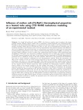
1.2 Pressure drop across the nasal cavity as a function of ﬂow rate 13

1.3

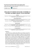
Inspiratory airﬂow streamlines in the nasal cavity with sinuses coloured by velocity from Tan et al. [2] . . . . . . . . . . . . . 14

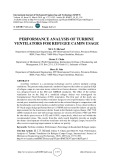
1.4 Velocity contours at the nasal valve for steady state inspiratory ﬂow rates of a) 7.5 lpm and b) 15 lpm from Wen et al. [3] . . 14

1.5 Schematic overview of research . . . . . . . . . . . . . . . . . . 18

2.1 Example of how greyscale values are assigned to pixels in a

CT image . . . . . . . . . . . . . . . . . . . . . . . . . . . . . 23

VIII

2.2 Flow chart showing the process by which an anatomical geom- etry is prepared - with the help of medical imaging software - for solution via CFD codes . . . . . . . . . . . . . . . . . . . . 26

2.3 Geometries of the ﬁve cavities used for analysis in this the- sis. The variation in smoothness is attributed partially to anatomical variations and partially to variations in reconstruc- tion methodology. . . . . . . . . . . . . . . . . . . . . . . . . . 28

2.4 Example of nasal cavity geometry generation: 2.4a shows an example of the extraction of a 3D model from CT scan data, using, in this case, an open source software package, slicer. Figure 2.4b shows the reﬁned geometry extracted from the CT slices seen in ﬁgure 2.4 (a) . . . . . . . . . . . . . . . . . . 29

2.5 Examples of the mesh types described in section 2.3.2 . . . . . 30

2.6 Example of mesh cell with spacing ∆x , ∆y and angle θ be- tween the grid lines along with high AR triangular and quadri- lateral elements . . . . . . . . . . . . . . . . . . . . . . . . . . 31

2.7 Mesh independence test carried out for the largest and smallest

of the new models presented in this thesis . . . . . . . . . . . 32

2.8 Average velocity in the sagittal plane as a function of nor- malised sagittal distance from the nostrils - up to the start of the nasopharynx - compared for the smallest and largest cavities presented in this thesis, for a range of mesh resolutions 33

2.9 Velocity contours at the nasal valve for three mesh resolutions

shown in 2.7 . . . . . . . . . . . . . . . . . . . . . . . . . . . . 34

2.10 Mesh of NC06 (68yo) . . . . . . . . . . . . . . . . . . . . . . . 35

3.1 Fluid moving through the computational domain, the inﬂow

of ambient air must be equal to the air entering the lungs . . . 40

3.2 Representation of mesh discretised with ﬁnite volume method 46

4.1 Direct comparison of WSS surface contours between all models 51

4.2 Coronal area weighted average of wall shear stress plotted as a function of distance from the entrance to the cavity across the sagittal axis . . . . . . . . . . . . . . . . . . . . . . . . . . 52

4.3 Peak velocity in the sagittal plane as a function of normalised sagittal distance from the nostrils, up to the start of the na- sopharynx . . . . . . . . . . . . . . . . . . . . . . . . . . . . . 53

4.4 Velocity contours and wall shear stress values along the perime- ter outlines of two cross-sections. The x-axis is the perime- ter distance starting from the top apex of each cross-section slice, and moves along the perimeter laterally. One full tracing around the perimeter is deﬁned as 1.0. The dashed line repre- sents the ﬂoor of the cross-section opposing its apex, and for the nasal valve, the halfway point 0.5, while for the turbinate cross-section it is 0.7. The y-axis represents wall shear stress normalised with respect to each individual slice’s maximum value0 − 1. . . . . . . . . . . . . . . . . . . . . . . . . . . . . . 55

4.5 Flow streamlines (coloured in blue) passing through the left and right chambers of the nasal cavity. Each chambers wall shear stress is shown (coloured in red). . . . . . . . . . . . . . 57

4.6 Streamlines through the cavities and sagittal contours taken at the nasal valve, turbinal region and choannae. Both are coloured by velocity magnitude, normalised with respect to each cavity’s maximum velocity. . . . . . . . . . . . . . . . . . 59

4.7 Colour coded display of the regional divisions used in tables

4.1, 4.2, 4.3 . . . . . . . . . . . . . . . . . . . . . . . . . . . . 60

4.8 Representation of the slicing method used for sampling data

across the sagittal axis throughout this thesis . . . . . . . . . 60

4.9 Cross sectional silhouettes taken at evenly spaced intervals across the sagittal axis of the cavities between the vestibule and nasopharynx . . . . . . . . . . . . . . . . . . . . . . . . . 61

4.10 Area versus distance across the four nasal cavities with a series

of examples from the literature . . . . . . . . . . . . . . . . . 62

4.11 Circularity factor versus normalised distance from the nostril inlet to the nasopharynx. This length for each model is: 48yo 8.97cm; 60yo 9.26cm; 64yo 9.60cm; 68yo 9.31cm; 78yo 8.45cm 65

4.12 Variation of pressure drop with ﬂow rate. A sample of results

from the literature is also included for comparison . . . . . . . 68

4.13 Static pressure versus normalised axial position across the ﬁve

nasal cavities . . . . . . . . . . . . . . . . . . . . . . . . . . . 69

4.14 Relative humidity as a function of normalised sagittal position 70

4.15 Average ambient temperature as a function of normalised sag-

gital position . . . . . . . . . . . . . . . . . . . . . . . . . . . 70

List of Tables

2.1 Parameters of the meshes for the nasal cavity models presented

in this thesis . . . . . . . . . . . . . . . . . . . . . . . . . . . . 36

4.1 Sectional volume, according to sections as seen in Figure 4.7

(cm3) . . . . . . . . . . . . . . . . . . . . . . . . . . . . . . . . 63

4.2 Sectional surface area, according to sections shown in Figure

4.7(cm2) . . . . . . . . . . . . . . . . . . . . . . . . . . . . . . 63

a (cm) . . . . . . . . . . . . . . . . . 64

4.3 Eﬀective diameter deﬀ = 4v

4.4 Minimal axial cross sectional area (cm2) . . . . . . . . . . . . 64

XII

Abstract

Older nasal cavities tend to exhibit a range of symptoms and pathologies more frequently than those of younger patients. These symptoms include variations in airconditioning functionality, as well as olfaction and mucosal clearance functionality. Several factors have been identiﬁed as potentially responsible for these symptoms. One issue that has been identiﬁed as a po- tential cause for a number of the identiﬁed symptoms is aberrations in airﬂow structures caused by age-related variations in nasal cavity anatomy. Various methods have been used to examine nasal patency between demographics, including Computational Fluid Dynamics (CFD) studies of airﬂow through nasal cavity models developed from Computed Tomography (CT) scans. To date CFD methods have not been used to examine airﬂow in older nasal cavities. This study will apply previously developed techniques for interde- mographic analysis to CFD simulation results from a series of older, Asian, adult male nasal cavity models.

Firstly the reconstruction methods used for creating the nasal cavity ge- ometries are detailed. The discretisation and setup of the CFD simulations carried out for the ﬁve models are then outlined. The results are then dis- cussed.

This study provides preliminary understanding connecting nasal anatomy, age and airﬂow dynamics. Although the study size was limited, it provides

insight into potential relationships between inhaled airﬂow characteristics and geometry. In particular discrepancies are noted in pressure drop, where the more voluminous cavities showed lower overall resistance: an overall pressure drop of 13 Pa was noted for the thinnest cavity as opposed to 2 Pa for the most voluminous; wall shear distribution, where the concentration at the nasal valve was signiﬁcantly reduced in the larger cavities: a peak of 0.16 Pa was noted for the thinnest cavity as opposed to 0.04 for the widest; as well as heat and vapour transfer, where higher volume cavities - in particular across the nasal valve - showed lower heat and vapour transfer rates. It is concluded that there are clear correlations between cavity volume and airﬂow characteristics within the nasal cavity.

Chapter 1 Introduction

1.1 Background

The ageing global population increases the need for investment in geriatrics. One area of particular signiﬁcance within this ﬁeld is that of rhinology. A range of dysfunctions and aberrations from the normal functioning of nasal cavities in healthy adults have been observed in the elderly population [4, 5]. For example, the occurrence of respiratory diseases in the elderly is markedly higher than that found in younger populations [6, 4]. It has been suggested that these higher recorded rates could be due in part to the impaired air conditioning functionality [5].

The nasal cavities of elderly citizens exhibit increased volume [7]. Alter- ations in histiological function have also been shown [6]. The extent to which functional aberrations are caused by geometric (as opposed to histiological) variations remains unclear [8]. These changes in nasal physiology - and their impact on nasal functionality - need to be investigated further.

Computational Fluid Dynamics (CFD) numerically approximates ﬂow ﬁeld characteristics for a given domain. CFD simulations give highly detailed results with information covering a range of areas for a given ﬂuid system at a minimal cost. One area in which CFD simulations have been gaining cre- dence is that of biomechanics; many biological ﬂuid systems can be modelled eﬀectively through CFD simulations, allowing for an unprecedented insight into their function.

The use of 3D medical imaging techniques such as computed tomography (CT) scans in collaboration with CFD has facilitated the numerical approxi- mation of ﬂuid mechanism parameters in anatomically accurate models. This allows for more detailed analysis of the eﬀects of topological variations on ﬂuid mechanisms. This capacity for detailed comparison makes CFD simu- lation an ideal tool for analysing the impact of physiological discrepencies on nasal patency.

To date numerous inter-demographic studies have been carried out using CFD analysis of 3D models reconstructed from CT scan data [9, 10, 11]. These studies have indicated that factors such as ethnicity and gender are liable to impact on nasal physiology. Previous studies have focused on age [9], however to date these age related studies have all focused on children. The use of CFD to examine functional variations in older models - accounting for potential interdemographic variations such as gender or ethnicity - is thus an important step that needs to be taken in order to achieve a more comprehensive understanding of the impact of ageing on nasal patency. For the sake of this thesis, the term older will be taken to mean ages of 60 and older.

Figure 1.1: Cross-section through the middle of the nasal cavity Showing the olfactory region (upper shaded area). NV, nasal vestibule; IT, inferior turbinate and oriﬁce of the nasolacrimal duct; MT, middle turbinate and oriﬁces of frontal sinus, anterior ethmoidal sinuses and maxillary sinus; ST, superior turbinate and oriﬁces of posterior ethmoidal sinuses [1]

1.2 Literature review

In this section the relevant literature regarding older nasal cavities will be reviewed. Signiﬁcant gaps in the current body of knowledge will be identiﬁed and serve as the foundation for this thesis.

1.2.1 Nasal cavity anatomy

The nasal cavity is the primary conduit for air coming into the respiratory system. [12]. The nasal cavity consists of two 5 by 10 cm chambers running between the nostrils and the pharynx [1]. The cavities are each made up

of three meatus. The meatus are connected to the nasolacrimal duct and paranasal sinuses, which are the largest of the many sinuses that surround the nasal cavity [1]. The nasal cavity is lined by respiratory epithelium. This epithelium controls the movement of mucous within the nasal cavity and is thus essential to its (the nasal cavity) airconditioning functionality [1]. The two major functions of the nasal cavities are conditioning of the air for interaction with the internal airways by warming and humidiﬁcation, and olfaction [13, 12, 1, 14].

1.2.2 Geriatric rhinology

Rhinology is the branch of medicine that deals with the nose and its patholo- gies. Common rhinological complaints of the elderly include dryness, runny noses, crusting and epistaxis [8]. Epidemiological studies have been carried out to examine the consistency of the manifestation of various symptoms throughout elderly patients with mixed results.

The literature at present seems to be unanimous on the tendency of the nasal cavity’s cross sectional area to increase with age. Several researchers have investigated this phenomena using acoustic rhinometry and shown good concordance in study outcomes [7, 4, 15, 5]. Loftus et al. [16] compared the volumes of 22 nasal cavity models taken from CT scan data, and also found a clear tendency towards increased nasal cavity volume with ageing. Nasal air heating and humidiﬁcation examined in vivo have been shown to be im- paired in older patients; Lindemann et al. [5] found average end-inspiratory temperature of 24◦C for older patients as opposed to 27.1◦C for younger patients. Their ﬁndings for humidity were comparable.

Increases in postnasal drip, nasal drainage, sneezing, coughing, olfactory dysfunction and gustatory rhinitis with age were observed in a clinical study

of 131 patients [4]. A 2009 study found that in a sample of 80 people no sig- niﬁcant relationship could be observed between age and nasal discomfort [17]. The same study, however, concurred with previous results on the increase of volume and cross sectional area as a function of age. Changes within the nose appear to not be limited to the increased volume; Both functional and structural variations in the respiratory epithelium have been observed with age, contributing to slower clearing of mucous [6].

Functional variations in air conditioning capabilities have been shown in vivo [5], with statistically signiﬁcant reductions in relative humidity and heat transfer observed in elder nasal cavities. The level to which this is attributable to change in histological function as opposed to variations in the ﬂuid mechanisms as a result of the expansion of the cavity remains to be investigated.

1.2.3 Experimental studies in rhinology

To investigate air ﬂow mechanisms in older nasal cavities, an experimental In this section the technique for the investigation must ﬁrst be chosen. methods available for investigating nasal patency are presented.

The anatomy of the nasal cavity was ﬁrst classiﬁed in detail by Emil Zuckerlandl in the 19th century [18]. Anatomically, his records were more or less up to the standard of what can be assessed from modern scanning techniques [18], however the investigation of airﬂow characteristics was still severely limited by technological capacity [19]. It was not until the turn of the 19th century that experimentation in to nasal airﬂow began in proper [19].

Some of the more common in vivo techniques used include rhinomanom- etry, which measures of the pressure drop across the nasal cavity [20]; and

acoustic rhinometry, which allows measurement of the cross sectional area of the nasal cavity as a function of depth [20].

Ultimately, however, direct detailed measurements of ﬂow mechanics within

the human nasal cavity taken in vivo are not practically viable with current technology as a result of the complexity and small scale of the nasal geometry [21]. Thus the preferred media for the testing in modern times has tended to be either physical or computational models reconstructed from CT scan data [21]. The physical models that have been constructed from CT scan data are able to provide detailed geometric reproductions. These geometries can then be used to create accurate 3D models which can then be used with techniques like particle image velocimetry to conduct in detailed ﬂow anal- ysis throughout the nasal cavity [22, 23]. These techniques allow for data about instantaneous velocities at many points throughout a working ﬂuid to be obtained through photographic methods. From this data the ﬂow regime can be computed with high accuracy, allowing for in depth quantitave and qualitative analysis. Spence et al. [24], for example, showed detailed velocity contours from unsteady ﬂow experiments using PIV. Such experimental set ups are, however, costly to run in terms of time and resources, in particular when compared with the high level of detail that can be achieved from a well done CFD simulation [25].

1.2.4 Computational studies

Background

Computational ﬂuid dynamics(CFD) is a discipline which is concerned with the computational approximation of solutions to the navier stokes equations for closed ﬂuid systems [26]. In many ﬁelds - inlcuding rhinology - CFD has facilitated economical and detailed investigations into cases in which

experimental investigation would otherwise be costly or impossible [27].

CFD was the primary driving force behind the development of larger and faster computers until the 80’s [28]. In more recent times, the continuing ad- vancement of computational technologies has facilitated considerable growth in the scope and accuracy of CFD for predicting the behaviour of increasingly complex systems [26].

Nasal airﬂow

One of the areas of investigation that has been facilitated by these advances is that of nasal airﬂow. Initially, simpliﬁed nasal cavity geometry models were used to create computational meshes and solve numerically for the ﬂuid ﬂow characteristics under steady state state conditions [27, 29]. Later 3D models extracted from CT scans were used to achieve more accurate results [30].

Boundary conditions

Various inlet and outlet conditions have been considered, including the dif- ference between unsteady state (ﬂowrate as a function of time throughout the nasal cycle) [31] and steady state (constant velocity, time independent) assumption based models [3]. This discrepancy has been a point of much contention, and it seems that the current position is that the correct choice depends on the application at hand [21]. Certainly to date it seems that the vast bulk of the case studies comparing diﬀerent geometries have used the steady state state assumption [9, 11, 10, 21, 27, 32, 3]. This assumption has been qualiﬁed on the basis of the low (below 0.2) Strouhal number for respi- ratory airﬂow [27], and more recently veriﬁed for certain parameters such as

wall shear stress [21].

The ﬂow rate for many of these steady state experiments and simulations has been determined on the basis of resting minute ventilation for healthy adults [32, 3]. This ﬁgure tends to be recorded around 7.5 litres per minute [33, 34]. This gives an average steady ﬂow inspiratory rate of 15 litres per minute (as the minute volume is both inhaled and exhaled during one round of respiration) [32]. For such ﬂow rates the ﬂow can be accurately treated as laminar [21, 29].

Another issue which has been of some debate in the literature is the rel- evance of the inclusion of sinuses in the modelled ﬂow domain. It has been reasonably commonplace to include the sinuses in studies that are examining the eﬀects of sinus surgery [35, 36]. Also it has been shown that, while the impact on airﬂow is relatively minimal, the sinuses can be subject to signiﬁ- cant levels of particle deposition for particles in the range of 1 nanometre in diameter, and particularly for low ﬂow rates [37]. The added requirements in time and computational complexity necessitated by the inclusion of the sinuses, however, seems to warrant their exclusion from models in situations where they are not speciﬁcally relevant [21].

Earlier numerical models restricted their domain to the nasal cavity itself [27, 32, 3]. Later it was suggested that the area around the nasal vestibule is liable to inﬂuence the developement of the inlet ﬂow distribution [13]. The facial features have also been shown to inﬂuence ﬂow ﬁeld developement [38]. More recently, facial features have been included in computational models to allow for inlet proﬁle developement [39, 40].

Older nasal cavities

Computational studies have yet to be undertaken for older nasal cavities. It is expected that the technologies available to us now for studying variations in nasal functionality could aﬀord an unprecedented insight into their structure and function.

1.2.5 Geometric variations

The basis of any in depth investigation into the relationship between geomet- ric variations and airﬂow structures is a clear analysis of the geometric vari- ations. Various demographic factors have been suggested to inﬂuence nasal morphology, such as ethnicity; as humans evolved, nasal cavities adapted to variations in climate as to preserve optimal heat and moisture exchange in the nasal mucosa [41, 42, 43, 44, 45].

Cross sectional areas have been graphed as a function of radial position to compare the geometries of diﬀerent models in many studies [9, 11, 5, 10]. Surface area has also been suggested to be signiﬁcant metric in predicting ﬂow behaviour (as surface area to volume ratios are expected to impact on the ﬂow behaviour) [9, 10]. The minimum coronal cross-sectional area is a ﬁgure that has been suggested to be of particular siniﬁcance to ﬂow development [5]. The ratio of area to volume (or perimeter length to cross sectional area) has been used by several researchers to predict ﬂow characteristics [9, 10].

The lack of detailed computer based studies to date on older models means that many of these metrics and investigative techniques, are yet to be applied to older models, despite the deeper insight into their functionality that they could provide.

1.2.6 Fluid dynamics

Pressure drop

Pressure drop across the nasal cavity is widely considered to be highly coro- lated with sensations of nasal patency [46]. The earliest papers investigating nasal patency focused primarily on the pressure drop over the nostrils, as measured with rhinomanometry [47]. Resistance across the nasal cavity, measured as pressure drop, is still often used as a predictor of ﬂow behaviour within the nasal cavity [4, 5, 15]. Pressure drop has also been suggested to provide insight in to the inspirational eﬃciency of the cavities [48]. It is often plotted as a function of ﬂow rate in order to provide a point for valida- tion by comparison with experimental set ups [3, 49]. In addition, it can be treated as a function of longitudinal position in order to gain an insight in to the relationship between the geometric variations and pressure drop [48]. A selection of distributions of pressure drop as a function of ﬂow rate, both experimentally and computationally determined, can be seen in Figure1.2.

Pressure drop across the nasal cavity is of particular interest in older cavi- ties, as computational analysis of the pressure drop across older cavities could assist in the understanding of the relationship between the rhinomanometry and acoustic rhinometry results for older cavities presented by previous re- searchers such as Lindemann et al. [5], who found for a transnasal pressure of 150 Pa that older patients exhibited an average ﬂow rate of 306cm3/s as opposod to 279 for younger models.

Wall shear stress and velocity

Velocity distributions in the nasal cavity play a signiﬁcant role in olfaction [50] and Particle ﬁltration [51, 52] as well as general understanding of nasal

Figure 1.2: Pressure drop across the nasal cavity as a function of ﬂow rate

function [27, 11, 48]. These can be examined by cross sectional zone by zone analysis [27, 11], which has been suggested to be useful for the measurement of the eﬃcacy of olfaction [11], or by longitudinal sections [48, 53].

It has been suggested that shear stress at the wall of the nasal cavity could impact on the complex multifarious histiological mechanisms contained in the nasal epithelium [54]. Distributions are analysed longitudinally [3] or around the cross sectional parameter of the relevant section of the nasal cavity [55].

These measurements (Wall shear and velocity) have been shown to be signiﬁcant for predicting heat and mass transfer characteristics [53], and as such their longitudinal and parametric distributions are signiﬁcant for un- derstanding the distribution of such mechanisms.

One common visualisation method is the use of streamlines (shown in Figure 1.3). Streamlines, often coloured by velocity [3, 11, 10], are useful

Figure 1.3: Inspiratory airﬂow streamlines in the nasal cavity with sinuses coloured by velocity from Tan et al. [2]

Figure 1.4: Velocity contours at the nasal valve for steady state inspiratory ﬂow rates of a) 7.5 lpm and b) 15 lpm from Wen et al. [3]

for showing ﬂow distribution as well as signiﬁcant recirculation zones [48, 56]. Another commonly used method, shown in Figure 1.4 is coronal cross sectional contours coloured by velocity. These contours may or not include streamlines to help highlight the presence of vortices in the ﬂow [3]. Another method, presented in Lintermann et al. [48] uses a vortex detection algorithm to trace the vortices present in the ﬂow structure. In Lintermann et al. [48], these are then coloured by variables related to turbulence and vorticity in order to provide a deeper insight in to the vortex structure and behaviour.

Heat and vapour transfer

The conditioning of inhaled air - by both humidiﬁcation and heating - in preparation for interaction with the sensitive tissues of the respiratory sys- tem is one of the primary functions of the nasal cavity [12]. Under standard atmospheric conditions, the air reaches an average temperature around 34◦C and humidity of 32 mgH2O/l by its entrance to the pharynx [57]. Intereth- nic variations in Nasal airconditioning eﬀectiveness have been observed and suggested to be linked to climate related evolutionary variations [45, 58]. Re- ductions in airconditioning functionality in older patients have been observed experimentally [5]. The average temperature of the respiratory epithelium during resting nose breathing has been found to be 32.6◦C [59].

Earlier investigations into the heat and vapour transport characteristics of the nasal cavity used a straight pipe model as a simpliﬁcation of the nasal cavity geometry [60]. The ﬁrst experiments involving real nasal cavity geometries were carried out in the 80s, using cast models taken from cadavers [61].

In vivo experiments into temperature variation across the nasal cavity have been done using various temperature measuring devices; modern exper-

iments have tended towards using thermocouples because they are small and respond quickly [12]. For measuring humidity in vitro, modern researchers have tended towards the use of capacitative humidity sensors [57]. Detailed proﬁles of temperature and humidity throughout the nasal cavity have been presented by several past researchers [57].

CFD has been used to simulate heat and vapour transfer in the nasal cavities with good accordance with experimental results [62]. Early simula- tions investigating heat and vapour transfer used a steady state assumption for inﬂow conditions [63]. Later, the eﬀect of the nasal cycle on tempera- ture distributions was investigated, showing signiﬁcant variations in the nasal temperature distributions throughout the nasal cycle [54]. For these simu- lations, the respiratory epithelium, which coats the majority of the nasal cavity, was assumed to be at 100% relative humidity, with the exception of the interior of the nostrils, for which there was zero water ﬂux [54].

Coronal cross section temperature contours have been used to visualise the distribution of temperature throughout the nasal cavity; this provides a clear method for visualising the distribution of temperature throughout the cross section [64]. Sagittal heat ﬂux contours have also been used to similar eﬀect [65]. Heat ﬂux, temperature, water ﬂux and humidity have all been mapped as functions of position across the sagittal axis in the nasal cavity [10, 65, 66]. The nasal valve has been noted from these observations to be a region of particular signiﬁcance to heat and vapour transfer mechanisms [65].

In vivo studies looking at older nasal cavities have shown them to exhibit a reduced humidifying and heating capacity [5]. Further investigations through computational methods into these variations could lead to more insight into the mechanisms underlying these discrepanies.

1.2.7 Demographic studies

One common application of CFD and ﬂuid dynamics in rhinology is to inves- tigate the eﬀects of interdemographic variations in nasal geometry on ﬂow features. The previously investigated demographics include ethnicity [11]; disease [10]; and age [9]. Age can be subclassiﬁed into children [9] and the el- derly [5]. Both child and older nasal cavities have been investigated through in vitro [67] and in vivo [7, 4, 15, 5] experimental techniques. Child models have also been investigated computationally [9]. The variations that have been observed in children’s nasal airway functionality has been suggested to be linked to particle ﬁltration ability [9]. It seems plausible that this eﬀect could be signiﬁcant also in the case of elderly models. It is to date, however, unknown as in depth computational studies investigating ﬂow ﬁeld variations in older models are yet be undertaken.

1.3 Summary

Throughout this section, we have seen that the nasal cavity is an important organ for airconditioning as well as olfaction. We have seen that there are an assortment of ailments related to this organ which eﬀect older patients in particular. It has been seen that there are clearly established trends between nasal cavit volume and age. We have examined the various methods available for examining the functionality of the nasal cavity. We have also looked at the use of ﬂuid dynamics for classifying and understanding the functionality and pathology of the nasal cavity.

Although various experimental techniques have been used historically in rhinology, none of them provide the same cost eﬀectiveness and level of de- tail which can be obtained through computational analysis of 3D models

Figure 1.5: Schematic overview of research

obtained from medical imaging. This method has been used extensively in recent years to examine various aspects of nasal cavity functionality, includ- ing interdemographic variations therein. These investigations have yielded multifarious insights into the various capacities of the organ. To date, to the best of my knowledge, the investigated demographics have not included older patients.

1.4 Literature gap

On the basis of the literature review presented above, the following gaps in the current body of knowledge seem signiﬁcant:

• Detailed analysis of geometric discrepencies between older nasal cavities

based on 3D scan models are yet to be carried out

• The correlations between geometric discrepencies in older nasal cavities and the airﬂow mechanisms induced in them through inspiration has yet to be analysed

• The eﬀect of geometric discrepencies between older nasal cavities on

heat and vapour transfer has yet to be assessed in detail

1.5 Research questions and objectives

In light of the information posed above, the following questions become per- tinent:

• How do variations in nasal cavity geometry in older Chinese Males inﬂuence the inhaled airﬂow mechanisms, contributing to respiratory ailments?

• How do the geometry variations impact on heat and vapour transfer

within the cavity, contributing to respiratory ailments?

To address these issues, the following objectives are outlined:

• Reconstruct a series of nasal cavity geometries from medical scans that represent a spread of geometric characteristics [such as volume and surface area] across the norm. The existing literature shows a clearly deﬁned relationship between age and volume: these models will serve as a representative sample of the older population to be analysed com- putationally.

• Model airﬂow across the series of reconstructed nasal cavities using CFD with a steady state assumption; deﬁning inlet conditions to ap- proximate a resting rate of respiration.

• Compare the simulation results between geometries. A variety of post processing methods are available to compare various aspects of ﬂuid me- chanic functionaility of nasal cavity models. The literature has shown clear discrepencies in the functionality of nasal cavities as a function of age; it is our intention through these measurements to examine in more detail the relationship between these variations and geometry.

• Compare with results from the literature.

1.6 Research overview

Medical image reconstruction technologies now allow researchers to recon- struct highly detailed, digital 3D representations of various anatomical struc- tures from ct scans. When coupled with CFD simulations, this presents an unprecedented capacity for in depth analysis of physiological ﬂuid ﬂow mech- anisms.

This study aims to use CFD analysis of CT scan data from the nasal cavities of a range of older Asian males to investigate the impact of geometric variations between older nasal cavities on the airﬂow structures and air- conditioning capacity of the nasal cavity. Air ﬂow mechanisms, heat transfer rates and humidiﬁcation eﬃcacy are analysed in order to arrive at a more precise understanding of the role of nasal geometry in the presentation of respiratory ailments.

This study represents, to the best of our knowledge, the ﬁrst in depth, mechanistic, computational study undertaken into the role of nasal geometry in common rhinological symptoms observed in older patients.

Chapter 2 Model reconstruction and meshing

2.1 Introducton

The ﬁrst step towards the computational analysis of older nasal cavities is the obtainment of computer models to describe their geometry. In this section the reconstruction process by which such computer models were obtained for the purpose of this thesis is explained.

2.2 Geometry

2.2.1 Introduction

The reconstruction of nasal cavity model computer models- including dis- cretisation - can be divided into 5 stages: image aquisition, data conversion, segmentation, reﬁnement and meshing. Firstly medical imaging technologies are used to extract a series of pixelated slices, in which the various materials which make up the human body can be identiﬁed by variation in greyscale measurements. These slices are then interpolated to create a 3D structure of voxels (the 3D equivalent of a pixel).

The reconstruction of the nasal cavity geometries can be very time con- suming and prone to human error. The improvement on and automation of the reconstruction process are areas of active research. This chapter presents an overview of the methods in current use for the various phases (mentioned above) by which a nasal cavity geometry is prepared for computational solu- tion.

2.2.2 Non-invasive medical imaging

There are various forms of medical imaging that can be used for the iden- tiﬁcation of the nasal cavity geometry. Here we brieﬂy overview Computed Tomography (CT), the form of medical imaging used for the nasal cavity geometries presented in this thesis.

CT scans use a series of x-rays taken at regular intervals within the re- gion of interest. x-ray scans use photons sent in beams through the region of interest; these photons interact diﬀerently with the material that they encounter depending on its density. Electronic detectors feed the photon

Figure 2.1: Example of how greyscale values are assigned to pixels in a CT image

pattern emitted from the body in question to a computer, which uses this information to create images. These images are made up of pixels which are each assigned a grey scale value based on their x-ray attenuation coeﬃcient. In medical imaging the Hounsﬁeld scale is used, whereas in image processing the greyscale is numbered from black to white between 0 to 255. Figure 2.1 shows an example of how greyscale values are assigned to pixels in a CT slice. Since the distance between the slices is known, each 2D can be given a depth element, transforming it into a 3D element known as a voxel. The voxels from all the slices put together create a 3D representation of the scanned area.

2.2.3 Image segmentation

Once the CT scan has been outputted as a series of voxels, the anatomical geometries relevant to the project at hand need to be extracted. To achieve this goal, the voxels that make up the relevant section of the data need to be identiﬁed somehow. This can be done manually - by going through the

many slices that make up the CT scan and identifying the relevant areas - however this process is extremely time consuming.

Numerous algorithms have been developed for the purpose of automating the process of image segmentation; all of which have certain advantages and disadvantages. For the most part these algorithms can be subsumed in to three categories, presented below (in order of increasing complexity):

Thresholding regions are identiﬁed and separated according their greyscale

value. This is the simplest algorithm for deﬁning regions.

Edge detection either local maxima of the ﬁrst derivative of intensity or zero values of the second derivative are used to identify region edges. Edge detection tends to reduce the noise when compared with thresh- olding

Region based regions are grown from the inside out. This produces more

coherent regions, but is unable to detect regions that are segregated.

These methods and many more exist and are in active development; many of them are available for free online. The implementation of such algorithms from ﬁrst principles, however is quite a complex procedure. Fortunately many of these algorithms have already been implemented in software packages - of which commercial and open source variations are available - which are speciﬁcally compiled for working with medical imaging outputs. In the case of the current thesis, the processes undertaken using the techniques described above is described in Figure 2.2

2.2.4 Preparation of model for meshing

Once the region in question has been extracted from the medical imaging output, it can be saved as some CAD format. There are certain criteria that need to be fulﬁlled by a CAD model before it can be read by 3D meshing software and used to create a mesh. It is often the case when the data is exported from the medical imaging software that it is ’dirty’; that there are contradictory or arbitrary elements in the geometry. These elements need to be removed through the use of CAD software before the geometry is suitable for the creation of a useable ’clean’ 3D mesh. The details of the process by which the geometry is prepared for meshing in the case of this thesis are described in Figure 2.2.

2.2.5 Summary

Anatomical geometry reconstruction - including that of the nasal cavity - begins with medical imaging of the area in question. The geometry is then extracted from the medical imaging data using one (or several) of the avail- able extraction algorithms outlined above. After extraction, cleaning of the geometry with CAD software is generally necessary to ensure that the geome- try is water-tight and ’clean’ before it can be meshed. This chapter has given an overview of some of the more pertinent methods in current use for the reconstruction of anatomical geometries from medical imaging data. Figure 2.4 shows an example of the construction process.

Figure 2.3 shows the models reconstructed for and used in this thesis. They have been labeled NC for nasal cavity plus a number. The ﬁrst cavity, NC04, is 48 years old and was reconstructed by a colleague earlier and used in this thesis as a comparison point for the older models. The other models are aged between 60 and 78. All of the models are of healthy Asian males.

Figure 2.2: Flow chart showing the process by which an anatomical geometry is prepared - with the help of medical imaging software - for solution via CFD codes

In this case we chose only healthy Asian males as to minimise the impact of demographic variations other than age on the presented geometries.

2.3 Meshing

2.3.1 Introduction

The Navier Stokes equations, upon which CFD is based (see chapter 3), are in many instances unable to be solved analytically. In order to approximate a solution to a given system, its geometry must be approximated, or discre- tised, as a series of points. The process by which these points are deﬁned and related to one another is known as meshing; this in itself is a complex dis- cipline under active research. In this chapter current methods are reviewed, and guidelines are given for developing quality meshes.

2.3.2 Mesh types

There are many types of mesh that can be employed; all of them have their own advantages and disadvantages.

Structured meshes are divided into segments of uniform size and shape. They are usually characterised by cells posessing either four nodal cor- ner points in two dimensions, or eight in three dimensions. The points are mutually orthogonal. Being deﬁned in this relatively simple way facilitates a higher level of computational eﬃciency. They are, however, limited in the level of structural complexity that they can accomodate.

Unstructured meshes The geometries encountered in the respiratory sys-

Figure 2.3: Geometries of the ﬁve cavities used for analysis in this thesis. The variation in smoothness is attributed partially to anatomical variations and partially to variations in reconstruction methodology. 28

(a)

(b)

Figure 2.4: Example of nasal cavity geometry generation: 2.4a shows an example of the extraction of a 3D model from CT scan data, using, in this case, an open source software package, slicer. Figure 2.4b shows the reﬁned geometry extracted from the CT slices seen in ﬁgure 2.4 (a)

tem are generally too complex to be eﬀectively discretised in a struc- tured manner; in cases such as these unstructured meshes can be used to acommodate the complexities of the given geometry. Unstructured meshes - usually constructed from triangles or tetrahedra - do not ﬁt a regular pattern, and they do not have coordinate lines corresponding to curvilinear directions. Because of this, the solving of computations over unstructured domains is generally more computationally inten- sive; however with modern advances in computers this has become less signiﬁcant an issue in many cases.

Hybrid meshes One disadvantage to the use of unstructured meshes is that they tend to show less accuracy near the wall. One commonly applied solution is the use of hexahedral elements near the wall, with the rest of the volume ﬁlled with unstructured - usually tetrahedral - elements. This method tends to improve the accuracy of near wall computations. One drawback of this method is that the prism layers can break down in the vicinity of excessively contoured walls. This problem needs to be monitored in the meshing process to avoid it impacting on mesh quality. In this study this is the mesh type that is employed as it provides the

(a) structured o-grid

(b) unstructured

Figure 2.5: Examples of the mesh types described in section 2.3.2

most accurate results for complex geometries such as the nasal cavity.

2.3.3 Meshing algorithms

There are various meshing algorithms available, each with its own strengths and weaknesses. For the purpose of this study, an octree algorithm was selected. Octree algorithms work by repeatedly dividing The volume in to smaller sections, until the given criteria, for example mesh size, is fulﬁlled. This method is generally considered to be a relatively simple but robust approach to mesh generation. One drawback, however is that it can cause irregular element distributions near the boundary.

2.3.4 Quality

The quality of a generated mesh is dependant on its warp angle, skewness and aspect ratio. For a quadrilateral cell, as shown in ﬁgure 2.6, the aspect ratio of the cell is deﬁned as AR = ∆y ∆x . Within the interior region, the AR should be maintained within the range 0.2 < AR < 5. This can be somewhat

Figure 2.6: Example of mesh cell with spacing ∆x , ∆y and angle θ between the grid lines along with high AR triangular and quadrilateral elements

relaxed, however, in the vicinity of the wall.

θideal

(see ﬁgure 2.6 for theta). Mesh skewness is deﬁned as the extent to which it deviates in shape from the ideal. This is a square for quadrilateral cells, or an equilateral triangle for triangle or tetrahedral cells. It is deﬁned for triangles and tetrahedrals as θideal−θactual

Many grid generation packages contain speciﬁc algorithms and/or func- tions for improving mesh quality. The gradient of mesh size variation should not exceed 1.2, as higher variations can cause problems in convergance.

2.3.5 Mesh independence

A signiﬁcant source of error in the solution of CFD problems is derived from the discretisation process; when a system is separated into a number of ﬁnite elements, for the purpose of numerical solution, the solution that is obtained from its solution is an approximation. It is necessary, then, to ascertain the required resolution, or mesh size, required to calculate a result that approx- imates the exact solution to a satisfactory degree of accuracy. This is done by means of a mesh independence test. This entails the monitoring of one

(a) NC05 (78yo)

(b) NC07 (64yo)

Figure 2.7: Mesh independence test carried out for the largest and smallest of the new models presented in this thesis

- or several - ﬂuid ﬂow parameters of interest to the study over a series of mesh resolutions for the relevant system. Independence is said to have been achieved when the eﬀect of mesh size on the selected ﬂow variable(s) has become suﬃciently insigniﬁcant.

Figure 2.7 shows the results from the mesh independence test conducted for smallest and the largest of the ﬁve models presented in this thesis. Here velocity [averaged across the domain of the interior of the nasal cavity be- tween the nostrils and the nasopharynx] and wall shear stress - two param- eters of interest in this study - were averaged across the cavity for constant ﬂow rates. In addition velocity contours were mapped through the nasal vestibule, a region of signiﬁcance for ﬂow development, and compared for the three mesh resolutions (see Figure 2.9 The results were compared for a series of simulations using consistent meshing approaches but varying the mesh resolution until the variation in results with mesh size was seen to taper oﬀ. From these results an optimal mesh size was determined for the models presented in this thesis.

(a) NC05

(b) NC07

Figure 2.8: Average velocity in the sagittal plane as a function of normalised sagittal distance from the nostrils - up to the start of the nasopharynx - compared for the smallest and largest cavities presented in this thesis, for a range of mesh resolutions

2.3.6 Meshing of the nasal cavity

Here we provide an overview of the meshing process applied to one of the nasal cavity models presented in this thesis. The process was the same for the other four models.

The system is divided in to three parts. The ﬁrst of these surrounds the facial geometry directly adjacent to the nostrils; this is to allow for the devel- opement of a more realistic inlet proﬁle. The second is the nasal cavity itself. The third section is an pipe-like extension from the exit of the nasopharynx; this allows for the developement of a more realistic outlet proﬁle, in a similar manner to the section around the inlet. This system can be seen in Figure 2.10 (a).

The three stages of mesh reﬁnement can be seen in Figure 2.10 (b); The mesh resolution is much coarser in the external domain, reﬁned closer to the inlet and then is most ﬁne in the cavity itself, the area of interest. Note the use of hybrid mesh, with internal tetrahedral elements and close to wall prism layers, shown clearly in Figure 2.10 (d). Prism meshes in the meshes

Figure 2.9: Velocity contours at the nasal valve for three mesh resolutions shown in 2.7

(b) Intersection of three mesh resolutions

(a) Whole system with face, extension from outlet and external zone

(d) Prism layer of cavity mesh

Figure 2.10: Mesh of NC06 (68yo)

in this model had thicknesses starting from around 0.1 mm.

Model Mesh size (×1e06) Sex Age Ethnicity

NC04 NC05 NC06 NC07 NC09 3.99 1.85 2.56 2.90 1.90 Male Male Male Male Male 48 Han Chinese 78 Han Chinese 68 Han Chinese 64 Han Chinese 60 Han Chinese

Table 2.1: Parameters of the meshes for the nasal cavity models presented in this thesis

Chapter 3 CFD fundamentals

3.1 Introduction

Once a 3D model has been developed and meshed, a variety of numerical paramaters and methods must be determined and utilised in order to ac- curately model the ﬂuid system. This chapter present an overview of the techniques used for modelling the ﬂuid systems deﬁned by the nasal cavity models reconstructed for this thesis.

3.2 Fluid Dynamics

The aim of CFD is to numerically solve the physical conservation laws of Newtonian physics:

• Conservation of mass

• The conservation of momentum (Newton’s second law, the rate of change of momentum equals the sum of forces acting on the ﬂuid);

• The conservation of energy (ﬁrst law of thermodynamics, the rate of change of energy equals the sum of rate of heat addition to and the rate of work done on the ﬂuid).

3.2.1 Mass conservation

The principle of conservation of mass is that, in a closed system, the mass remains constant. This means that ﬂuid will move through a set region in such a way that the mass is conserved. For an incompressible ﬂow, this means that the outﬂows and the inﬂows will be equal. For a steady state system this can be written as

out

0 = (cid:88) ˙m − (cid:88) ˙m (3.1)

Where ˙m = mass ﬂow rate.

The mass ﬂow rate can be written as ρuA, for ρ = density, u = velocity and A is the scross sectional area of the ﬂow. For ﬂow in the x direction, A = ∆z∆x. For a two dimensional ﬂow, ∆z = 1, giving:

(3.2) ˙min = ρu∆y

Extending this to equation 4.3, in the x direction, for an incompressible

ﬂow we get

(3.3) 0 = ρuin∆yin − ρuout∆yout

This can easily be extrapolated to three dimensions.

Extending this further, in the x direction for the same two dimensional

element we can say that

∆x]∆y (3.4) ˙mout = [ρu + ∂(ρu) ∂x

Applying this in the y direction and substituting back into Equation 4.3,

for an incompressible ﬂow we get

0 = [ρu + ∆x]∆y − ρu∆y + [ρv + ∆y]∆x − ρv∆x (3.5) ∂(ρu) ∂x ∂(ρv) ∂y

which then simpliﬁes to

+ (3.6) 0 = ∂(ρu) ∂x ∂(ρv) ∂y

which is the continuity equation, and can easily be extended into three

dimensions as

0 = (3.7) + + ∂(ρu) ∂x ∂(ρv) ∂y ∂(ρw) ∂z

In the case of the nasal cavity, this can be conceptualised in relation to the nasal cavity geometry, where the air ﬂow rate going into the nostrils must be equal to that leaving through the extension from the nasopharynx, as seen

Figure 3.1: Fluid moving through the computational domain, the inﬂow of ambient air must be equal to the air entering the lungs

in ﬁgure 3.1.

3.2.2 Momentum conservation

(cid:80) F = ma

Momentum conservation is based on the Newton’s second law:

Here m is the mass of the system, a is its rate of acceleration, and (cid:80) F is the sum of forces acting on the system. F can generally be divided into body and surface forces. Rewriting the mass as the product of volume and the density, and acceleration as the ﬁrst derivative of velocity

(cid:88) Fbody + (cid:88) Fsurf ace = (ρ∆x∆y∆Z)

(3.8) DU Dt

Body forces generally include gravity, centrifugal, Coriolis and electro-

magnetic forces; these all act on the volume from a distance.

Surface forces are those that act directly on the surface of a ﬂuid element. These ﬂuid forces include normal stress, in the x direction σxx, which is

made up of pressure forces p exerted on the body and normal viscous stress components τxx; and tangential stresses, τxy and τxz.

Summing these forces in the x direction, for a 2D ﬂuid element we get

(cid:88) Fsurf ace,x = [σxx∆y∆z − ( ∂τyx ∂y

∆x)∆y∆z] ∂σxx ∂x (3.9) + [(τxy + ∆y)∆x∆z − τyx∆x∆z]

= − ∆x∆y∆z + ∆x∆y∆z ∂σxx ∂x ∂τyx ∂y

Assuming that the ﬂuid is Newtonian and isotropic, σxx can be related

to pressure p and viscous stresses τxx by

σxx = −p + τxx

For a Newtonian ﬂuid, stress-strain relations can be described as

(3.10) τxx = 2µ τyx = µ ∂u ∂x ∂u ∂y

Where µ is the viscocity of the ﬂuid. Combining equations 3.8 , 3.9 and

3.10 in the x direction, and cancelling out the volume term

(3.11) ρ = − + µ( Du Dt ∂p ∂x ∂2u ∂x2 + ∂2u ∂y2 ) + ρ (cid:88) Fb

Here the acceleration term is the total derivative of u, deﬁned as the combined local and advection inertial forces, which in two dimensions can be written as

= + v + u (3.12) Du Dt ∂u ∂t ∂u ∂y ∂u ∂x

combining equations 3.11 and 3.12 and dividing through by ρ

(cid:125)

(cid:124)

(cid:123)(cid:122) convection

(cid:123)(cid:122) dif f usion

+v + u = − + ν( ∂2u ∂x2 + ∂2u ∂y2 ) ∂u ∂y (cid:124) ∂u ∂x (cid:125) + (cid:88) Fb (cid:124) (cid:123)(cid:122) (cid:125) bodyf orce ∂u ∂t (cid:124)(cid:123)(cid:122)(cid:125) local acceleration ∂p 1 ρ ∂x (cid:124) (cid:123)(cid:122) (cid:125) pressuregradient (3.13)

Where ν is kinematic viscocity, deﬁned as µ ρ .

3.2.3 Energy Conservation

Conservation of energy is derived from the ﬁrst law of thermodynamics, that in a steady ﬂow system the total energy of a control volume remains constant; that inﬂows and outﬂows must be equal. This can be expressed analogously to the mass conservation as

(3.14) = (cid:88) ˙Q + (cid:88) ˙W DE Dt

Where ˙Q is heat transfer and ˙W is the rate of work done. E is energy

per unit mass and is expressed as

DE Dt can be expressed similarly to Equation 3.12

E = CpT

= + v + u + v + u ) (3.15) = Cp( DE Dt ∂E ∂t ∂E ∂y ∂T ∂t ∂T ∂y ∂T ∂x ∂E ∂x

For a 2D element, the total energy can therefore be calculated from

+ v + u )∆x∆y (3.16) ρ ∆x∆y = ρCp( DE Dt ∂T ∂t ∂T ∂y ∂T ∂x

From Fourier’s law of heat conduction, for a 2D system we can write

(3.17) = ˙qxAx = ˙qx∆y ˙Qx = kAx ∂T ∂x

where ˙q is heat ﬂux = ˙Q/A

The heat transferred into the element can thus be expressed as

= k (3.18) [qx + ]∆y − qx∆y = ∂qx ∂x ∂2T ∂x2 ∆x∆y ∂qx ∂x

reconstructing equation 3.14 with the inclusion of 3.18, considered also

in the y direction, we can cancel out the volume term

(cid:124)

(cid:125)

(cid:123)(cid:122) convection

(cid:123)(cid:122) dif f usion

+ v + u = ( (3.19) ∂T ∂x ∂2T ∂x2 + ∂2T ∂y2 ) ∂T ∂y (cid:125) k ρCp (cid:124) ∂T ∂t (cid:124)(cid:123)(cid:122)(cid:125) local acceleration

3.3 Humidity

One of the primary functions of the nasal cavity is the humidiﬁcation of the incoming air in preparation for its interaction with the lungs. any investi- gation into the ﬂuid mechanisms of the nasal cavity would be incomplete without adressing the eﬃcacy of this function.

All air has some water content. The amount of water content that air is capable of holding varies as a function of temperature and pressure. The ratio of the amount of water vapour present in a body of air to the maximum quantity that it (the body of air) is capable of holding is referred to as relative humidity. This is a commonly used metric for describing the vapour content of air.

One simple but eﬀective method for approximating humidiﬁcation data

in a computational domain is the use of the convection-diﬀusion equation.

Analogously to equations 3.19 and 3.13, for a 2D element we can write

(cid:125)

(cid:124)

(cid:123)(cid:122) convection

(cid:123)(cid:122) dif f usion

+ u + v (3.20) = DH2O( ∂Φ ∂x ∂2Φ ∂x2 + ∂2Φ ∂y2 ) ∂Φ ∂y (cid:125) ∂Φ ∂t (cid:124)(cid:123)(cid:122)(cid:125) localacceleration

Where Φ is the concentration of water vapour and DH2O is the diﬀusivity

of water in air.

In the commercial software package used for the solution of the models presented in this thesis (FLUENT), this is solved in the following form for laminar ﬂows:

(3.21) Ji = −ρDi,m∇Yi − DT,i ∇T T

Where Ji is the diﬀusion ﬂux of species i (in this case H2O), Di,m is the

mass diﬀusion coeﬃcient and DT,i is the thermal diﬀusion coeﬃcient.

3.4 Solving the governing equations

The conservation equations outlined earlier in this chapter are nonlinear par- tial diﬀerential equations which, for complex domains such as the nasal cavity geometry, have no analytical solution; they must therefore be approximated algebraically and solved numerically.

3.4.1 Discretisation

Approximating, or discretising a system to make it numerically solvable can be done in many ways. One of the more common methods in modern solvers is the ﬁnite volume method, which can be applied to unstructured as well as structured meshes, making it particularly suited to complex geometries such as that of the nasal cavity.

The Finite Volume Method discretises the system into a series of volumes. The ﬂuxes of relevant variables through the diﬀerent faces of each element are then treated as a discrete system, which is able to be solved numerically.

Discretisation methods can be characterised according to the order of ap- proximation. Higher order approximations will provide more accurate results but can be in some cases more diﬃcult to solve.

Finite volume methods can tend to cause artiﬁcial, or numerical, diﬀusion if the mesh is of low quality. It is thus necessary to follow proper meshing practices, similar to those outlined in section 2.3.

Figure 3.2: Representation of mesh discretised with ﬁnite volume method

3.4.2 Numerical Solution

Once the system has been discretised, a system of linear equations can be developed to describe the system. These equations can be solved with one of several methods. These methods can generally be divided into two categories: either direct or iterative. In general, for large complex domains such as the nasal cavity models presented in this paper, iterative methods are the only way to derive a solution.

In order to solve the equations satisfactorily for incompressible ﬂows an extra term must be added in order to obtain values for pressure. This is called pressure-velocity coupling. The method used for pressure velocity coupling in this thesis is the SIMPLE method, one of the most common methods available, the details of which can easily be found in any modern textbook on CFD.

Iterative solutions approximate a solution to the system of equations step by step. As the solution converges towards the desired state, the discrepancy between results for successive steps reduces. It is by monitoring these dis- crepancies, or residuals, that one determines when a solution has reached a satisfactory level of accuracy.

3.5 Setup and solution of nasal cavity models

used in this thesis

Here an overview will be given of the way that the solution of the nasal cavity systems presented in this thesis will be given. Firstly the models are prepared and meshed as discussed in the Chapter 2. Once this is done the boundary conditions for the system must be deﬁned.

The face and internal wall of the nasal cavity and pipe extension are set to no slip condition. This means that velocity is assumed to be zero on the sur- face of these zones. In order to maximise comparability between the models a constant inspiratory ﬂow rate is chosen for all the models; in reality rates of respiration vary signiﬁcantly between individuals, however in this case an assumed consistency of ﬂow rate increases our ability to compare the ﬂow characteristics between the models. To this eﬀect the exit of the pipe exten- sion is given a constant velocity value calculated for each model as to give an inspiritory ﬂow rate of 10 lpm, which has been suggested by the literature to be a realistic approximation for an inspiratory rate of an adult human at rest [3, 32]. For these simulations this ﬂow rate is treated as constant and the ﬂow treated as steady, an assumption which greatly simpliﬁes the solution process and one which is commonly used when comparing ﬂuid ﬂow characteristics between nasal cavity models (transient, or time dependant solutions are computationally much more costly). The 3D incompressible navier stokes equations were solved iteratively via the SIMPLE method for pressure-velocity coupling and a second order upwind scheme for convection.

The border of the hemispheric region around the face is set to atmospheric pressure. For resting inspiratory ﬂow rates ﬂow within the nasal cavity has been shown to be modelled most accurately as laminar [13, 29]; as such no turbulence model is used.

The temperature of the air coming from the outside is set to 20◦C and the wall temperature inside the nasal cavity is set to 32.6◦C. The species mass fraction of H2O to give 100% relative humidity at the cavity wall is calculated for 32.6◦C, with the exception of the nasal vestibule, where diﬀusive ﬂux is set to zero. The species mass fraction of H2O for the air coming into the model is calculated to give a relative humidity of 45% for 101.3 kpa and 20◦C.

The numerical solution of the systems - described by the aforementioned boundary conditions and meshes - is approximated, for the models of this thesis, by the use of a commercial CFD code, in this case ANSYS FLUENT. The following chapter details the analysis of the solutions obtained for the ﬁve cavities.

Chapter 4 Results

4.1 Introduction

A large amount of information can be obtained from the results of a thor- ough CFD simulation. The challenge then becomes to present it in a way that is clear and comprehensible. This chapter presents the analysis of the simulation results for the ﬂuid systems deﬁned by the nasal cavity models reconstructed for the thesis.

4.2 Wall shear stress and velocity

Figure 4.5 shows ﬂow streamlines through the left and right nasal chambers with the chambers wall shear stress. In all the models ﬂow acceleration and high wall shear stresses were consistently found in the region between the nasal vestibule entrance (anterior) and before the middle nasal passage. We also note that there is a preference for the streamlines to pass through the

mid-height of the nasal chambers. A small fraction reached the olfactory region, and some inferiorly along the ﬂoor of the chambers. The highest wall shear stress values were found in the 48yo, 60yo, and 78yo models which are also the models with the smaller cross-sectional area proﬁles (from Figure 4.10), and corresponds to the highest velocity magnitudes produced by the streamlines in the models. Wall shear stress contours viewed from the top and lateral left-chamber side of all nasal models are shown in Figure 4.1. By using the same colour scale the results show directly the disparity between nasal models.

Figure 4.1 shows the wall shear stress across the ﬁve models presented in this paper. The valve region can be seen to be a region of particularly high wall shear across all the models. Also note that the distributions of wall shear vary signiﬁcantly in the more voluminous cavities

From Figure 4.2, wall shear stress can be seen to be more pronounced in general in the less voluminous models such as the 48yo, and in particular this eﬀect is exaggerated in the valve region. Here the wall shear stress is mapped from the nostrils to the entrance of the nasopharynx. The nasophar- ynx showed more pronounced variations, in particular the 48yo showed a sig- niﬁcant spike in wall shear stress in the nasopharynx, which is to be expected because of its lower cross sectional area. Note that the sagittal distribution of wall shear stress is much more even in the larger cavities. The valve region - considered of particular signiﬁcance to the development of ﬂow features within the nasal cavity [5] shows signiﬁcant variation in wall shear stress concentration, with the 64yo and 60yo presenting a very even distribution of wall shear stress, in contrast to the 48yo or 78yo which show wall shear more pronounced around the opening from the vestibule. Similar variations can also be seen in the distribution within the turbinal region (Figure 4.1).

In Figure 4.3 The peak velocity in the sagittal plane is shown in as a

Figure 4.1: Direct comparison of WSS surface contours between all models

Figure 4.2: Coronal area weighted average of wall shear stress plotted as a function of distance from the entrance to the cavity across the sagittal axis

function of normalised sagittal distance from the nostrils in Figure 4.3. The ﬂow development region is diﬀerent in the thinner cavities. Also the inlet region seems to have an impact on the ﬂow through the whole cavity, as you can see particularly in NC09, because it has a wider valve and narrower turbinal region, but the maximum velocity stays consistently low despite the lower cross sectional area in the turbinal region, suggesting a strong correlation between vestibule cross sectional area and ﬂow development. This supports theories put forward by Doorly et al. [21] on the importance of the nasal valve on ﬂow development.

Cross-sections at the internal nasal valve, and turbinate region were taken for each model and its velocity contour presented in Figure 4.4. We traced the perimeter of each cross-section starting from its apex and follow down in a counter-clockwise direction. For the nasal valve cross-section in all models, we found that the surface proportion was distributed almost evenly between

Figure 4.3: Peak velocity in the sagittal plane as a function of normalised sagittal distance from the nostrils, up to the start of the nasopharynx

the lateral and septum walls. This is observable in the fact that the separa- tion point between the lateral and septal walls (as annotated on ﬁgure 4.4) occurred at 0.5. For the turbinate region, this occurred at 0.7 meaning that 70% of the perimeter resides along the lateral side and 30% of the perimeter is along the septum wall. Here the septal wall is deﬁned as the part of the cavity directly adjacent to the septum, and the lateral wall as the remainder. For the 48yo model we labelled three peaks for the nasal valve slices (r1, r2, and l1) to help identify the locations on the cross-section itself.

Wall shear stress peaks occurred close to the regions of maximum veloci- ties in the contours. Superiorly, where the velocity is very low, the wall shear stress is nearly zero. These peaks and troughs correlate well with the contour slices and is consistent for all models.

In Figure 4.6 Streamlines are shown through the nasal chambers, coloured

Figure 4.4: Velocity contours and wall shear stress values along the perimeter outlines of two cross-sections. The x-axis is the perimeter distance starting from the top apex of each cross-section slice, and moves along the perimeter laterally. One full tracing around the perimeter is deﬁned as 1.0. The dashed line represents the ﬂoor of the cross-section opposing its apex, and for the nasal valve, the halfway point 0.5, while for the turbinate cross-section it is 0.7. The y-axis represents wall shear stress normalised with respect to each individual slice’s maximum value0 − 1.

Figure 4.5: Flow streamlines (coloured in blue) passing through the left and right chambers of the nasal cavity. Each chambers wall shear stress is shown (coloured in red).

by velocity. In addition Sagittal contours of the vestibule, turbinal region and choannae are included.

4.3 Geometry Variations

One-hundred cross-sectional slices were taken from the nostrils tip to the nasopharynx. From nostrils tip to choanae, vertical slices were made, while angled slices were made in the nasopharynx until the slice became horizontal (Figure 4.8).

Figure 4.9 shows 8 coronal slices taken at equidistant spacing across the sagittal axis between the anterior vestibule and the nasopharynx. We see the airway elongate vertically which increases the perimeter length while maintaining a relatively constant surface area. This area to perimeter ratio has been cited as an important factor in the development of ﬂuid ﬂow in the nasal cavity [10, 9]. The thinner cavities also tend to exhibit higher wall shear stress. This is because of the steeper velocity gradients, which create stress through the viscosity of air, near the wall. This narrowness is also likely to inﬂuence heat and vapour transfer in the cavities; when the cavities are narrower there is less distance for the heat and vapour to travel from the wall to saturate the incoming air, and so it is likely to saturate the airﬂow more comprehensively. The variation in cavity thickness between the cavities can also be clearly observed in this ﬁgure.

Figure 4.10 shows the cross sectional area as a function of normalised distance along the sagittal axis. The distance has been normalised between the entrance to the nostrils and the end of the nasopharynx. A sample of cavities from the pre-existing literature has also been included for compari- son. A signiﬁcant variation can be seen in the average cross sectional area of the models presented in this paper; This variation is most pronounced

Figure 4.6: Streamlines through the cavities and sagittal contours taken at the nasal valve, turbinal region and choannae. Both are coloured by velocity magnitude, normalised with respect to each cavity’s maximum velocity.

Figure 4.7: Colour coded display of the regional divisions used in tables 4.1, 4.2, 4.3

Figure 4.8: Representation of the slicing method used for sampling data across the sagittal axis throughout this thesis

Figure 4.9: Cross sectional silhouettes taken at evenly spaced intervals across the sagittal axis of the cavities between the vestibule and nasopharynx

Figure 4.10: Area versus distance across the four nasal cavities with a series of examples from the literature

towards the rear of the cavities. None of the models show quite the same volume as the atrophic rhinitis model, also shown here as Garcia [10], prior to the nasopharynx, although the 64yo is close. The general shape of the curve is reasonably similar for the various models in this paper, with notable exceptions in the Nasopharynx of the 64yo cavity and a larger spike in the vestibule region of the 78yo. Observations from Figure 3 can be compared with the cross sectional silhouettes from Figure 2, for a clearer understanding of the variations in geometry between the 4 models presented here. The range of cross-sectional areas allows us to observe the relationship between various ﬂuid mechanical properties of the cavity and cavity volume/cross-sectional area.

Table 4.1 - 4.3 shows the variation of the volume, surface area and eﬀective diameter respectively, in comparison with models from the literature. The

48yo, NC04 18.54 78yo, NC05 22.78 68yo, NC06 24.62 64yo, NC07 30.722 60yo, NC09 16.73 Xi al. [9] 12.63 Garcia et al.[10] 33.66

5.40 12.80 20.09 4.57 16.33 10.60 3.84

4.15 32.33 2.81 40.23 4.21 55.07 7.39 28.69 5.50 34.43 2.41 47.77 Turbinal region Naso- pharynx Vestibule 3.10 25.48 Total

Table 4.1: Sectional volume, according to sections as seen in Figure 4.7 (cm3)

48yo, NC04 170.92 78yo, NC05 174.07 68yo, NC06 190.44 64yo, NC07 163.44 60yo, NC09 138.80 Xi al. 112.59 Garcia et al. 133.501

12.20 12.80 25.23 40.42 11.37 40.93 31.46

Turbinal region Naso- pharynx vestibule 15.71 198.82 total 17.37 204.25 12.45 228.11 17.92 221.79 46.96 197.192 35.58 189.10 - 164.96

Table 4.2: Sectional surface area, according to sections shown in Figure 4.7(cm2)

volumes of the four models presented in this paper varied signiﬁcantly. The largest discrepancies were noted in the pharynx and turbinate regions, with a less marked discrepancy in the vestibular region. The 48 yo is showing greater volume than that seen in the atrophic rhinitis patient from [10]. The surface area of the atrophic rhinitis model is also signiﬁcantly lower, to the extent that the eﬀective diameter, shown in Table 4.3, is larger than the models presented in this paper.

Minimal cross sectional area, shown in Table 4.4, is signiﬁcant to ﬂow across the cavity[5]. Here the atrophic rhinitis model shows larger minimal cross sectional area than any of those found in the models presented here, although it is quite close to that of the 64yo.

48yo, NC04 0.434 78yo, NC05 0.52 68yo, NC06 0.52 64yo, NC07 0.75 60yo, NC09 0.48 Garcia et al. 1.11 Xi al. 0.45

1.26 1.69 2.03 1.99 1.61 1.35 1.60

Turbinal region Naso- pharynx vestibule 0.79 0.51 total 0.96 0.63 0.90 0.71 0.94 0.99 0.63 0.58 - 1.13 0.62 0.72

a (cm)

Table 4.3: Eﬀective diameter deﬀ = 4v

et Garcia et al. 48yo, NC04 1.665 78yo, NC05 3.0174 68yo, NC06 1.80 64yo, NC07 4.14 60yo, NC09 2.7 Xi al. Unknown 3.04 MCA

Table 4.4: Minimal axial cross sectional area (cm2)

The circularity shape factor (a dimensionless quantity used in image anal- ysis) was used to quantify the cross-sectional shape (Figure 4.11). The cir- cularity, fo , (also known as the isoperimetric quotient), is the ratio of cross- sectional area bounded by a closed curve, to its perimeter deﬁned as,

(4.1) fo = 4πA P 2

At the nostril inlet, the circularity ranges from 0.18-0.30 and this reduces to a value of approximately = 0.035 (except the 64yo model). It then in- creases rapidly towards 1 where the two nasal chambers merge and form a single conduit in the form of the nasopharynx.

Figure 4.11: Circularity factor versus normalised distance from the nostril inlet to the nasopharynx. This length for each model is: 48yo 8.97cm; 60yo 9.26cm; 64yo 9.60cm; 68yo 9.31cm; 78yo 8.45cm

4.4 Pressure drop

The pressure drops across the nasal cavities can also be seen in Figure 4.12 to vary in relation to the volume of the nasal cavity. This is in contrast to the experimental ﬁndings of [5, 4, 15], whose studies using rhinomanometry showed no signiﬁcant decrease in pressure across the cavity to accompany the recorded variation in volume. The cause of this discrepancy is unclear. Its presence is, however, supported by pipe ﬂow theory. Starting with the Bernoulli equation for pressure drop ∆P

(4.2) ∆P = ρ × loss = γhf

where hf is frictional headloss and γ = ρg.

Pressure drop can be written as

)(ρV 2) (4.3) ∆P = 2f ( L D

πD2 and f is the friction factor = 16

Re for

where V is volume ﬂow rate = 4Q

πDν . Therefore

laminar ﬂow, where Re = 4Q

∆P = (4.4) 8πDν Q L D 16ρQ2 π2D4

cancelling out gives

∆P = 128 (4.5) ρνLQ πD4

ρ, ν, L, Q and π are more or less constant between the models, so then

we expect to see an correlation of

∆P ∝ (4.6) 1 D4

this means that for a twofold variation in equivalent diameter, such as that seen between NC04 and NC07 for example, we would expect to see a sixteenfold discrepancy in pressure drop across the cavity for laminar ﬂow, which is slightly less than is observed here (17.38 and 0.93 Pa respectively). However, when taking into consideration the increased pressure head loss in NC04 due to the rapid reduction in diameter at the exit from the nasophar- ynx, this ﬁgure seems very close to that which would be predicted analyti- cally. Although the correlation between the pipe ﬂow theory presented above and nasal cavity ﬂuid dynamics is limited due to the complexities of nasal cavity geometry, the above formulae none the less support the viability of the results obtained through the simulations presented in this thesis. In ad- dition, Edelstein et al. [4] showed a large range of pressure drops in their study using rhinomanometry, many of which showed variations of compara- ble magnitude. Also Garcia et al. [10] and Kelly et al. [68] showed similar relationships between pressure and cavity volume (both of these are included in Figure 4.12).

Figure 4.13 shows pressure drop as a function of normalised sagittal loca- tion across the nasal cavity. Here the pressure drop is primarily seen across the valve region. Here the nasopharynx has been excluded from the domain; the signiﬁcant pressure drop across the nasopharynx was inversely propor- tional to the cross sectional areas of the respective nasal cavities

Figure 4.12: Variation of pressure drop with ﬂow rate. A sample of results from the literature is also included for comparison

Figure 4.13: Static pressure versus normalised axial position across the ﬁve nasal cavities

4.5 Heat and vapour transfer

Some variation in the heat and vapour transfer eﬃcacy can be seen between the models presented in this thesis. Note the higher than average ﬁgures for temperature and relative humidity in the valve area of the 78yo. In general the more voluminous models exhibit lower humidity and temperature (Figures 4.14 and 4.15). The data from the atrophic rhinitis study by Garcia et al [10] is also included for comparison. Clearly the impact of the geometric variations associated with atrophic rhinitis on heat and vapour transfer are much more pronounced than that of the more voluminous older cavities when compared with the thinner cavities presented here.

Figure 4.14: Relative humidity as a function of normalised sagittal position

Figure 4.15: Average ambient temperature as a function of normalised sag- gital position

Chapter 5 Discussion

Evaluation of nasal respiratory function for diagnostic or research purposes relies on categorisation of an individual’s demographics, including age, gen- der, and ethnicity. It is known that normal changes in inter- or intra- individual nasal cavities manifest through age. This is especially true of intranasal volume, which is thought to increase due to hormonal changes [5] leading to mucosal atrophy [7, 17]. Edelstein [4] and Lindemann et al. found correlations between aging and the occurrence of a range of rhinolog- ical conditions (e.g. dry cold itchy noses; crusting, postnasal dripping and obstructed nasal breathing) although their association with nasal morphol- ogy was not established. Thus, a detailed analysis of the nasal morphology and its eﬀect on respiratory function in older adult patients may contribute towards this understanding.

Demographic factors such as age, gender, and ethnicity play an impor- tant role in determining ones nasal anatomy and physiology. For example, it was found that males exhibited larger nasal cavities e.g. larger normal pharyngeal areas in males over females [69, 70]. However, very few studies

have quantiﬁed these diﬀerences. In terms of geometric variations with age, Kalmovich, et al. [7] found a signiﬁcant increase in nasal cavity volume and minimal cross sectional area with age using acoustic rhinometry on 165 pa- tients. Later, Lindemann, et al. [17] used acoustic rhinometry in conjunction with rhinomanometry and validated questionnaires to survey the nasal cavi- ties of eighty patients. While the questionnaire and rhinomanometry did not show any diﬀerence between the older and younger subjects, a marked in- crease in the volume of the nasal cavity with age was found from the acoustic [16] found higher intranasal rhinometry data. More recently, Loftus, et al. volumes with age on CT volumetric analysis.

In the past, quantifying diﬀerences in nasal airﬂow has been limited by a lack of sensitive tools that can quantify the complexities of the sinonasal cavity. More recently, CFD has been proven to be a useful tool for detailed analysis of nasal airﬂow. With this new tool, normative data based on demo- graphics is required so that these can be compared with disease states. We aimed at investigating the nasal airﬂow anatomy and physiology of older Chi- nese adult males to understand geometry features and dynamics of inhaled ﬂow ﬁeld in this speciﬁc demographic group.

Our geometry analyses revealed the signiﬁcant inﬂuence of the area to perimeter ratio on ﬂuid ﬂow development in the nasal cavity. The thinner cavities exhibited higher wall shear stresses due to sharper velocity gradients that were produced. The narrow geometry would also increase heat and vapour transfer as there is less distance for the heat energy and vapour to transport from the wall to condition the inhaled air.

The cross-sectional area of slices taken along the nasal cavity, provided insight into the patients airway patency based on the degree of openness of the nasal chamber. These observations (from Figure 4.10) can be compared with cross sectional outlines in Figure 4.9 which allow predictions of the

likely relationships between ﬂuid ﬂow properties caused by the individual nasal geometry features.

A shape factor in the form of the circularity, described the overall shape of each cross-sectional slice along the nasal cavity geometry. A circularity of 1 implies a circular shape, although this can be masked by irregular shapes that coincidently have the same values as a smooth circle. A value close to zero, however is more deﬁnite providing a strong suggestion of a jagged and non- circular shape. The sharp increase in the circularity plot indicated where merging of the two chambers occurs. The circularity is a well-established measurement commonly used in image analysis of particles, and this is the ﬁrst time it has been applied for shape detection in nasal cavity geometries. The results in this study showed that circularity is useful as an indicator and quantiﬁable metric for identifying the anterior, middle, and posterior nasal cavity regions.

Fluid ﬂow analysis showed the relationship between inhaled ﬂuid dynam- ics and its impact on ﬂuid-surface shear. Regions of high acceleration were often caused by the airway converging into a smaller cross-section thereby ac- celerating the ﬂow through. This corresponded with a high wall shear stress region in the vicinity of the minimised cross-section.

The pressure drop across the cavities as a function of volume was sup- ported by pipe ﬂow theory analytically, and the level of variation observed is not excessive when compared with the level of variance seen in previous stud- ies using rhinomanometry [4]. The relationship between volume and pressure drop is interesting, however, as it is not seen in previous studies examining relationships between aging, volume and pressure drop [5]. This is likely re- lated to the limitations of acoustic rhinometry in measuring cavity volume past the turbinal region of the nasal cavity. Experimental validation of the pressure drops across the models presented in this study would go further to

conﬁrm this theory.

The 48yo and 60yo models were the smallest in size and this resulted in higher wall shear stress magnitudes. Based on the geometry analysis, peak velocities and wall shear stresses should occur at the minimal cross-sections, and this corroborated well with the highest values indeed found in the 48yo and 60yo models. Locally, the highest wall shear stress concentrations oc- curred around the internal nasal valve, and this is consistent across all the models. Interestingly the nasopharynx also exhibited a signiﬁcant increase in wall shear stress, and this was due to the cross-sectional area decreasing at the nasopharynx. The inﬂuence of nasal valve geometry on ﬂow development is clearly seen, particularly in NC09 which exhibits an expanded nasal valve. As a result the peak velocity in the turbinal region is lower in comparison to the sections cross sectional area when compared with the other models pre- sented here. The wall shear stress proﬁles along cross-sectional slices showed peak wall shear stresses produced inferiorly on the internal nasal valve while there was very low wall shear stresses superiorly. For the turbinate slices, the velocity contours showed the bulk ﬂow and peak velocity were oﬀset from the nasal ﬂoor. This is the continuation of the ﬂuid ﬂow that was rising from the nasal valve region. The main nasal passage expands but the ﬂow is unable to reach the new extremities.

The static pressure variation shown in Figure 4.13 merits some discussion. Although it would seem logical that an increased cavity volume would have the eﬀect of reducing pressure drop, this is not the result that has been recorded by previous researchers using rhinomanometry [5]. This discrepancy is possibly due to the ﬂexibility of the soft palate, varying the diameter of the exit in ways that are not replicated in the CT models. The eﬀect of the soft palate on the aperture of the exit from the nasal cavity will inﬂuence ﬂow separation in the nasopharynx. This is also a contributing factor in total static pressure drop across the cavity. The geometry of the nasal cavities also

plays a role in the static pressure drop across the cavity by inﬂuencing ﬂow features [71]. For example by creating ﬂow separation points which increase resistance [71].

The more even distribution of wall shear stress - both sagittally, as seen in Figures 4.1 and 4.2; and coronally, as seen in Figure 4.4 - is indicative of variations in airﬂow structure and therefore performance of the nasal cavity models; the higher wall shear is a direct result of sharper velocity and pressure gradients near the wall [72]. In particular the variation in the local maxima for WSS found in the region of the nasal valve is indicative of varying air conditioning capacity.

It seems in particular that it is only in the more severely enlarged cavities that drastically increased ﬂow recirculation is seen in the air ﬂow structures (as can be observed in Figure 4.6).

It seems probable that these marked increases in recirculation are linked to the observed reductions in air-conditioning functionality in specimens from this age group [73]. This is in accordance with the ﬁndings of [10] in relation to atrophic rhinitis patients. The model in their study had a recorded volume of 34.5 cm3, however this was only measured to the end of the septum, and a comparison with the models from this study, as seen in Figure 4.10 shows that the volume through the turbinal region of the atrophic rhinitis model was signiﬁcantly larger than that of the largest model from this study, NC07. Although a quantity is not given for the volume of the nasopharynx in the atrophic rhinitis model, qualitative comparison between the images of the model and those of the models from this study seem to show that the signiﬁcant expansion of the nasopharynx which is present in all of the elderly models was not present in the model of the younger (26 yo) atrophic rhinitis suﬀerer.

Previous research has suggested that the presence of signiﬁcant vortices

such as those seen in the larger of the models presented in this study is related to the impairment of air conditioning functionality. The speciﬁcs of this mechanism , however, are yet to be investigated, and this is a piece of work which should be completed in future. In addition, the impact of the observed variations in airﬂow structure on the ability of the nasal cavity to ﬁlter particles from the air has not been investigated, and this is also an area which could be of some signiﬁcance.

The heat and vapour transfer ﬁgures show what seems to be close to an inverse linear relationship between the voluminousness of the cavities and their heat and vapour transfer eﬃcacy. This is particularly pronounced in the nasal valve. This relationship agrees well with the data from Garcia et al [10] taken from their atrophic rhinitis patient. This suggests that the mechanisms causing this reduced eﬃcacy in the atrophic rhinitis patient are the same as those in elderly patients; this may imply that, for more extreme cases, that the surgical procedures implemented for atrophic rhinitis patients could also be eﬀective for the elderly. It has been suggested by [5] that heat and vapour transfer are signiﬁcantly eﬀected by the minimal cross sectional area. The current data doesn’t show anything to support or disprove this suggestion, as in general the models presenting higher MCAs are also presenting higher voluminousness. In fact, the model that shows the highest MCA relative to its voluminousness [NC09], shows very good heat and vapour transfer.

Detailed understanding of the associations among variabilities in nasal anatomy, age, and airﬂow dynamics will greatly improve current knowledge regarding the inﬂuence of conductive mechanisms on olfactory ability. Vari- abilities in nasal anatomy have traditionally been understood to inﬂuence olfaction [74, 75]. Nasal proﬁles that have been postulated to be associated with improved olfaction include the dorsal conduit, which delivers inhaled odorant-laden air to the olfaction recess through enhanced olfactory airﬂow, and an enlarged olfactory recess at the posterior end of the nasal cavity

[74, 75, 76]. It has also been reported that anatomical changes in the olfac- tory cleft or the nasal valve region alter odorant transport to the olfactory epithelium [77]. Furthermore, the incidence of olfactory dysfunction in the general population is unclear, but has been estimated to be between 1% and 3%, with an exponential increase of 24.5% among individuals aged 53 to 97 years [78, 79, 80, 81, 82]. The present study provides preliminary under- standing connecting nasal anatomy, age and airﬂow dynamics together.

5.1 Conclusions

Aberrations in nasal cavity form and functionality associated with the ageing process are important issues. Their importance is growing as the global pop- ulation ages. The underlying mechanisms behind many nasal cavity patholo- gies associated with the ageing process are still largely unknown.

This thesis presents ﬁndings from a set of preliminary investigations into in to older nasal cavity anatomy and airﬂow characteristics. Although the sample size here is limited, it provides some preliminary insights in to ques- tions raised by previous experimental results looking at the eﬀects of old age on nasal cavity geometry and airﬂow.

In particular it provides a clear mechanistic alternative take on the rela- tionship between geometry and nasal resistance to that provided by previous investigations using rhinomanometry and acoustic rhinometry. These (rhi- nomanometry and acoustic rhinometry) results show no clear relationship between cavity volume and resistance, whereas our computational investiga- tion shows a clear relationship. Although a deﬁnitive answer is not oﬀered as to the nature of the observed discrepency in ﬁndings, it does serve to identify the lack of understanding of this area in the current literature.

This thesis also provides a ﬁrst look at mechanistic variations in older nasal cavity airﬂow, as well as previously unseen details regarding geometric formations. A circularity factor is introduced to quantify variations in shape between cavities for the anterior, middle and posterior nasal cavity regions.

Signiﬁcant variations in ﬂow concentration and developement are seen between the more and less voluminous cavities, particularly in regions - such as the nasal valve - cited as being of particular signiﬁcance to ﬂow devel- opement. The impact of this on ﬂow developement is clearly seen in Figure 4.3, where a clear relationship is seen between valve cross sectional area and overall peak velocity.

Preliminary examinations are made into heat and vapour transfer within the cavities; The results suggest some relationship between geometry and these functions in the nasal cavity.

5.2 Future works

The ﬁrst gap left answered by this thesis is as to the validity of the results for the more voluminous cavities. Although the results make sense when compared with previous results from rhinomanometry, as well as pipe ﬂow theory, for completeness the results should be validated experimentally.

Another signiﬁcant area which should be investigated is the impact of the aberrations observed in this thesis on particle deposition zones in the nasal cavity. This area is signiﬁcant for both olfaction and particle ﬁltration. It is the hope and intention of the author of this thesis that the preliminary insights presented here will lay the groundwork for future developments in the ﬁeld of geriatric rhinology.

Bibliography

[1] Niels Mygind and Ronald Dahl. Anatomy, physiology and function of the nasal cavities in health and disease. Advanced Drug Delivery Reviews, 29(12):3 – 12, 1998. Nasal Drug Delivery.

[2] Jie Tan, Demin Han, Jie Wang, Ting Liu, Tong Wang, Hongrui Zang, Yunchuan Li, and Xiangdong Wang. Numerical simulation of normal nasal cavity airﬂow in chinese adult: a computational ﬂow dynamics model. European Archives of Oto-Rhino-Laryngology, 269(3):881–889, 2012.

[3] Jian Wen, Kiao Inthavong, Jiyuan Tu, and Simin Wang. Numerical simulations for detailed airﬂow dynamics in a human nasal cavity. Res- piratory Physiology & Neurobiology, 161(2):125–135, 2008.

[4] David R. Edelstein. Aging of the normal nose in adults. The Laryngo-

scope, 106(S81):1–25, 1996.

[5] Joerg Lindemann, Diana Sannwald, and Kerstin Wiesmiller. Age re- lated changes in intranasal air conditioning in the elderly. Laryngoscope, 118:1472–1475, 2008.

[6] James Ho, Kwok Chan, Wayne Hu, Wah Lam, Ling Zheng, George Tipoe, June Sun, Raymond Leung, and Kenneth Tsang. The eﬀect of aging on nasal mucociliary clearance, beat frequency, and ultrastructure

of respiratory cilia. American Journal of Respiratory and Critical Care Medicine, 163(4):983–988, Mar 2001.

[7] L. M. Kalmovich, D. Elad, U. Zaretsky, A. Adunsky, A. Chetrit, S. Sadetzki, S. Segal, and M. Wolf. Endonasal geometry changes in elderly people: Acoustic rhinometry measurements. Journals of Geron- tology Series a-Biological Sciences and Medical Sciences, 60:396–398, 2005.

[8] Victoria E Varga-Huettner and Jayant M Pinto. Physiology of the aging nose and geriatric rhinitis. In Nasal Physiology and Pathophysiology of Nasal Disorders, pages 165–181. Springer, 2013.

[9] Jinxiang Xi, Ariel Berlinski, Yue Zhou, Bruce Greenberg, and Xiawei Ou. Breathing resistance and ultraﬁne particle deposition in nasal- laryngeal airways of a newborn, an infant, a child, and an adult. Annals of Biomedical Engineering, 40:2579–2595, 2012.

[10] Guilherme J. M. Garcia, Neil Bailie, Dario A. Martins, and Julia S. Kimbell. Atrophic rhinitis: a cfd study of air conditioning in the nasal cavity. Journal of Applied Physiology, 103(3):1082–1092, 2007.

[11] Jian Hua Zhu, Heow Pueh Lee, Kian Meng Lim, Shu Jin Lee, and De Yun Wang. Evaluation and comparison of nasal airway ﬂow patterns among three subjects from caucasian, chinese and indian ethnic groups using computational ﬂuid dynamics simulation. Respiratory Physiology & Neurobiology, 175(1):62–69, 2011.

[12] David Elad, Michael Wolf, and Tilman Keck. Air-conditioning in the hu- man nasal cavity. Respiratory Physiology & Neurobiology, 163(1-3):121 – 127, 2008. Respiratory Biomechanics.

[13] D. Doorly, D.J. Taylor, P. Franke, and R.C. Schroter. Experimental

investigation of nasal ﬂow. Proc. of the Institution of Mechanical Engi- neers Part H - J Engineering in Medicine, 222(H4):439–453, 2008.

[14] B. Berglund and T. Lindvall. Olfaction, pages 279–306. Elsevier Biomed-

ical Press, New York, 1982.

[15] Si Whan Kim, Ji-Hun Mo, Jeong-Whun Kim, Dong-Young Kim, Chae- Seo Rhee, Chul Hee Lee, and Yang-Gi Min. Change of nasal function with aging in korean. Acta Oto-Laryngologica, 127(S558):90–94, 2007.

[16] Patricia A Loftus, Sarah K Wise, Daniel Nieto, Nicholas Panella, Ashley Aiken, and John M DelGaudio. Intranasal volume increases with age: Computed tomography volumetric analysis in adults. The Laryngoscope, 2016.

[17] Joerg Lindemann, Evangelia Tsakiropoulou, Iordanis Konstantinidis, and Kerstin Lindemann. Normal aging does not deteriorate nose-related quality of life: Assessment with nose and snot-20 questionnaires. Auris Nasus Larynx, 37:303–307, 2010.

[18] H Stammberger. History of rhinology: anatomy of the paranasal sinuses.

Rhinology, 27(3):197–210, 1989.

[19] R. Eccles. Nasal airﬂow in health and disease. Acta Oto-Laryngologica,

120(5):580–595, 2000.

[20] O. Hilberg, A. C. Jackson, D. L. Swift, and O. F. Pedersen. Acoustic rhinometry: evaluation of nasal cavity geometry by acoustic reﬂection. Journal of Applied Physiology, 66:295–303, 1989.

[21] D. J. Doorly, D. J. Taylor, and R. C. Schroter. Mechanics of airﬂow in the human nasal airways. Respiratory Physiology & Neurobiology, 163(13):100–110, 2008.

[22] S.K. Chung and S.K. Kim. Digital particle image velocimetry studies of nasal airﬂow. Respiratory Physiology & Neurobiology, 163(1-3):111–120, 2008. doi: DOI: 10.1016/j.resp.2008.07.023.

[23] J.T. Kelly, A.K. Prasad, and A.S. Wexler. Detailed ﬂow patterns in the

nasal cavity. J Appl. Physiol., 89:323–337, 2000.

[24] C. J. T. Spence, N. A. Buchmann, and M. C. Jermy. Unsteady ﬂow in the nasal cavity with high ﬂow therapy measured by stereoscopic piv. Experiments in Fluids, 52(3):569–579, 2012.

[25] Baoshun Ma, Vincent Ruwet, Patricia Corieri, Raf Theunissen, Michel Riethmuller, and Chantal Darquenne. Cfd simulation and experimental validation of ﬂuid ﬂow and particle transport in a model of alveolated airways. Journal of Aerosol Science, 40(5):403–414, 2009. doi: DOI: 10.1016/j.jaerosci.2009.01.002.

[26] J. Tu, G.H. Yeoh, and C. Liu. Computational ﬂuid dynamics: a practical

approach. Butterworth-Heinemann, 2008.

[27] K Keyhani, PW Scherer, and MM Mozell. Numerical simulation of airﬂow in the human nasal cavity. Journal of biomechanical engineering, 117(4):429–441, 1995.

[28] J.F. Wendt and J.D. Anderson. Computational ﬂuid dynamics: an in-

troduction. Springer, 2009.

[29] I. Hahn, P.W. Scherer, and M.M. Mozell. Velocity proﬁles measured for airﬂow through a large-scale model of the human nasal cavity. J Appl. Physiol., 75(5):2273–2287, 1993.

[30] T. B. Martonen, Z. Zhang, G. Yue, and C. J. Musante. 3-d particle transport within the human upper respiratory tract. Journal of Aerosol Science, 33(8):1095–1110, 2002.

[31] H. Shi, C. Kleinstreuer, and Z. Zhang. Laminar airﬂow and nanoparticle or vapor deposition in a human nasal cavity model. Journal Biomech. Eng., 128(5):697–706, 2006.

[32] R.P. Subramaniam, R.B. Richardson, K.T. Morgan, J. S. Kimbell, and R.A. Guilmette. Computational ﬂuid dynamics simulations of inspira- tory airﬂow in the human nose and nasopharynx. Inhalation Toxicology, 10(91-120), 1998.

[33] MS Chaya, AV Kurpad, HR Nagendra, and R Nagarathna. The eﬀect of long term combined yoga practice on the basal metabolic rate of healthy adults. BMC complementary and alternative medicine, 6(1):1, 2006.

[34] M J Tobin, T S Chadha, G Jenouri, S J Birch, H B Gazeroglu, and M A Sackner. Breathing patterns. 1. normal subjects. Chest, 84(2):202–205, 1983.

[35] G. Xiong, J. Zhan, K. Zuo, J. Li, L. Rong, and G. Xu. Numerical ﬂow simulation in the post-endoscopic sinus surgery nasal cavity. Medical and Biological Engineering and Computing, 46(11):1161–1167, 2008.

[36] Joerg Lindemann, Hans-Juergen Brambs, Tilman Keck, Kerstin M. Wiesmiller, Gerhard Rettinger, and Daniela Pless. Numerical sim- ulation of Ameri- intranasal airﬂow after radical sinus surgery. doi: DOI: can Journal of Otolaryngology, 26(3):175–180, 2005. 10.1016/j.amjoto.2005.02.010.

[37] Qin Jiang Ge, Kiao Inthavong, and Ji Yuan Tu. Local deposition frac- tions of ultraﬁne particles in a human nasal-sinus cavity cfd model. In- halation Toxicology, 24(8):492–505, 2012.

[38] T.R. Anthony, M.R. Flynn, and A. Eisner. Evaluation of facial features on particle inhalation. Annals of Occupational Hygiene, 49(2):179–193, 2005.

[39] Xiangdong Li, Kiao Inthavong, and Jiyuan Tu. Particle inhalation and deposition in a human nasal cavity from the external surrounding envi- ronment. Building and Environment, 47(0):32–39, 2012.

[40] Jong-Hoon Lee, Yang Na, Sung-Kyun Kim, and Seung-Kyu Chung. Un- steady ﬂow characteristics through a human nasal airway. Respiratory Physiology & Neurobiology, 172(3):136–146, 2010.

[41] Arthur Davies. A re-survey of the morphology of the nose in relation to climate. The Journal of the Royal Anthropological Institute of Great Britain and Ireland, 62:337–359, 1932.

[42] Arthur Thomson. Man’s nasal index in relation to certain climatic con- ditions. The Journal of the Royal Anthropological Institute of Great Britain and Ireland, 53:92–122, 1923.

[43] J.S. Weiner. Nose shape and climate. Am J Phys Anthropol, 12:1–4,

1954.

[44] S. Churchill, L.L. Shackelford, N. Georgi, and M. Black. Morphological variation and airﬂow dynamics in the human nose. Am J Human Biol, 16:625–638, 2004.

[45] Marlijn L. Noback, Katerina Harvati, and Fred Spoor. Climate-related variation of the human nasal cavity. American Journal of Physical An- thropology, 145(4):599–614, 2011.

[46] Giancarlo Ottaviano and WJ Fokkens. Measurements of nasal airﬂow and patency: a critical review with emphasis on the use of peak nasal inspiratory ﬂow in daily practice. Allergy, 71(2):162–174, 2016.

[47] R Martin, PS Vig, and DW Warren. Nasal resistance and vertical dento- facial features. In Journal of Dental Research, volume 60, pages 539–539, 1981.

[48] Andreas Lintermann, Matthias Meinke, and Wolfgang Schrder. Fluid mechanics based classiﬁcation of the respiratory eﬃciency of several nasal cavities. Computers in Biology and Medicine, 43(11):1833 – 1852, 2013.

[49] Kiao Inthavong, Man Chiu Fung, Xuwen Tong, William Yang, and Jiyuan Tu. High resolution visualization and analysis of nasal spray drug delivery. Pharmaceutical research, pages 1–8, 2014.

[50] Shigeru Ishikawa, Toshio Nakayama, Masahiro Watanabe, and Teruo Matsuzawa. Flow mechanisms in the human olfactory groove: Numeri- cal simulation of nasal physiological respiration during inspiration, expi- ration, and sniﬃng. Arch Otolaryngol Head Neck Surg, 135(2):156–162, 2009.

[51] K. Inthavong, Z. F. Tian, H. F. Li, J. Y. Tu, W. Yang, C. L. Xue, and C. G. Li. A numerical study of spray particle deposition in a human nasal cavity. Aerosol Science and Technology, 40(11):1034–1045, 2006.

[52] S. M. Wang, K. Inthavong, J. Wen, J. Y. Tu, and C. L. Xue. Comparison of micron- and nanoparticle deposition patterns in a realistic human nasal cavity. Respiratory Physiology and Neurobiology, 166(3):142–151, 2009.

[53] D. J. Taylor, D. J. Doorly, and R. C. Schroter. Inﬂow boundary proﬁle prescription for numerical simulation of nasal airﬂow. Journal of The Royal Society Interface, 7:515–527, 2010.

[54] David Elad, Sara Naftali, Moshe Rosenfeld, and Michael Wolf. Phys- ical stresses at the air-wall interface of the human nasal cavity during breathing. Journal of Applied Physiology, 100(3):1003–1010, 2006.

[55] M.A. Burgos, E. Sanmiguel-Rojas, A. Martn-Alcntara, and M.L Hidalgo-Martnez. Eﬀects of the ambient temperature on the airﬂow

International Journal for Numerical

across a caucasian nasal cavity. Methods in Biomedical Engineering, 30(3):430–445, 2014.

[56] Jinxiang Xi, JongWon Kim, Xiuhua A. Si, Wei Chung Su, and Yue Zhou. Eﬀects of the facial interface on inhalation and deposition of Inhalation micrometer particles in calm air in a child airway model. Toxicology, 26:492–505, 2014.

[57] T. Keck, R. Leiacker, A. Heinrich, S. Kuhneman, and G. Rettinger. Hu- midity and temperature proﬁles in the nasal cavity. Rhinology, 38(167- 171), 2000.

[58] Todd R Yokley. Ecogeographic variation in human nasal passages.

American journal of physical anthropology, 138(1):11–22, 2009.

[59] J. Lindemann, R. Leiacker, G. Rettinger, and T. Keck. Nasal mucosal

temperature during respiration. Clin. Otolaryngol, 27:135–139, 2002.

[60] Sven Ingelstedt and Nils Gunnar Toremalm. Air ﬂow patterns and heat transfer within the respiratory tract: A new method for experimental studies on models. Acta Physiologica Scandinavica, 51(2-3):204–217, 1961.

[61] ML Nuckols, JL Zumrick, and CE Johnson. Heat and water vapor transport in the human upper airways at hyperbaric conditions. Journal of biomechanical engineering, 105(1):24–30, 1983.

[62] J. Lindemann, T. Keck, K. Wiesmiller, B. Sander, H.J. Brambs, G. Ret- tinger, and P. Pless. A numerical simulation of intranasal air tempera- ture during inspiration. The Laryngoscope, 114:1037–1041, 2004.

[63] S. Naftali, R.C. Schroter, J. Shiner, and D. Elad. Transport phenomena in the human nasal cavity: A computational model. Annals of Biomed- ical Engineering, 26:831–839, 1998.

[64] S. Naftali, M. Rosenfeld, M. Wolf, and D. Elad. The air-conditioning capacity of the human nose. Annals of Biomedical Engineering, 33:545– 553, 2005.

[65] Corbin D Sullivan, Guilherme JM Garcia, Dennis O Frank-Ito, Julia S Kimbell, and John S Rhee. Perception of better nasal patency corre- lates with increased mucosal cooling after surgery for nasal obstruction. Otolaryngology–Head and Neck Surgery, pages 139–47, 2013.

[66] Shen Yu, Xiu-zhen Sun, and Ying-xi Liu. Numerical analysis of the relationship between nasal structure and its function. The Scientiﬁc World Journal, 2014.

[67] I. Weinhold and G. Mlynski. Numerical simulation of airﬂow in the human nose. European Archive Otorhinolaryngology, 261:452–455, 2004.

[68] J.T. Kelly, B. Asgharian, J.S. Kimbell, and Wong. B.A. Particle depo- sition in human nasal airway replicas manufactured by diﬀerent meth- ods. part 1: Inertial regime particles. Aerosol Science and Technology, 38(11):1063–1071, 2004.

[69] J. Huang, H. Shen, M. Takahashi, T. Fukunaga, H. Toga, K. Takahashi, and N. Ohya. Pharyngeal cross-sectional area and pharyngeal compli- ance in normal males and females. Respiration, 65(6):458–68, Nov 1998. Copyright - Copyright (c) 1998 S. Karger AG, Basel; Last updated - 2011-04-05.

[70] Lee J Brooks and Kingman P Strohl. Size and mechanical properties of the pharynx in healthy men and women. The American Review of Respiratory Disease, 1992.

[71] Vaibhav H. Ramprasad and Dennis O. Frank-Ito. A computational anal- ysis of nasal vestibule morphologic variabilities on nasal function. Jour- nal of Biomechanics, 49(3):450 – 457, 2016.

[72] Kiao Inthavong, Yidan Shang, and Jiyuan Tu. Surface mapping for visualization of wall stresses during inhalation in a human nasal cavity. Respiratory Physiology & Neurobiology, 190:54–61, 2014.

[73] Joerg Lindemann, Evangelia Tsakiropoulou, Tilman Keck, Richard Leiacker, and Kerstin M. Wiesmiller. Nasal air conditioning in rela- tion to acoustic rhinometry values. American Journal of Rhinology & Allergy, 23(6):575–7, 11 2009. Copyright - Copyright OceanSide Publi- cations Nov 2009; Last updated - 2012-03-03.

[74] Thomas P Eiting, J Blair Perot, and Elizabeth R Dumont. How much does nasal cavity morphology matter? patterns and rates of olfactory airﬂow in phyllostomid bats. Proceedings of the Royal Society of London B: Biological Sciences, 282(1800):20142161, 2015.

[75] Brent A Craven, Thomas Neuberger, Eric G Paterson, Andrew G Webb, Eleanor M Josephson, Edward E Morrison, and Gary S Settles. Recon- struction and morphometric analysis of the nasal airway of the dog (canis familiaris) and implications regarding olfactory airﬂow. The Anatomical Record, 290(11):1325–1340, 2007.

[76] Thomas P Eiting, Timothy D Smith, J Blair Perot, and Elizabeth R Dumont. The role of the olfactory recess in olfactory airﬂow. Journal of Experimental Biology, 217(10):1799–1803, 2014.

[77] Kai Zhao, Peter W. Scherer, Shoreh A. Hajiloo, and Pamela Dalton. Ef- fect of anatomy on human nasal air ﬂow and odorant transport patterns: Implications for olfaction. Chem. Senses, 29(5):365–379, 2004.

[78] B N Landis, C G Konnerth, and T Hummel. A study on the frequency

of olfactory dysfunction. The Laryngoscope, 114(10):1764–1769, 2004.

[79] Annika Br¨amerson, Leif Johansson, Lars Ek, Steven Nordin, and Mats

Bende. Prevalence of olfactory dysfunction: The sk¨ovde population- based study. The Laryngoscope, 114(4):733–737, 2004.

[80] Charles J Wysocki and Avery N Gilbert. National geographic smell survey: eﬀects of age are heterogenous. Annals of the New York Academy of Sciences, 561(1):12–28, 1989.

[81] Howard J Hoﬀman, Erick K Ishii, and Robert H Macturk. Age-related changes in the prevalence of smell/taste problems among the united states adult population: Results of the 1994 disability supplement to the national health interview survey (nhis). Annals of the New York Academy of Sciences, 855(1):716–722, 1998.

[82] Claire Murphy, Carla R Schubert, Karen J Cruickshanks, Barbara EK Klein, Ronald Klein, and David M Nondahl. Prevalence of olfactory impairment in older adults. Jama, 288(18):2307–2312, 2002.