Nguyễn Công Phương
CONTROL SYSTEM DESIGN
The Performance of Feedback Control Systems
Contents
Introduction
I. II. Mathematical Models of Systems III. State Variable Models IV. Feedback Control System Characteristics V. The Performance of Feedback Control Systems VI. The Stability of Linear Feedback Systems VII. The Root Locus Method VIII.Frequency Response Methods IX. Stability in the Frequency Domain X. The Design of Feedback Control Systems XI. The Design of State Variable Feedback Systems XII. Robust Control Systems XIII.Digital Control Systems
sites.google.com/site/ncpdhbkhn
2
The Performance of Feedback Control Systems
1. Introduction 2. Test Input Signals 3. Performance of Second – Order Systems 4. Effects of a Third Pole & a Zero on the Second –
Order System Response
5. The s – Plane Root Location & the Transient
Response
6. The Steady – State Error of Feedback Control Systems 7. Performance Indices 8. The Simplification of Linear Systems 9. System Performance Using Control Design Software
sites.google.com/site/ncpdhbkhn
3
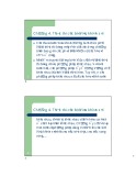
Introduction
Performance measure, M1
Performance measure, M2
pmin
Parameter, p
sites.google.com/site/ncpdhbkhn
4
The Performance of Feedback Control Systems
Introduction
1. 2. Test Input Signals 3. Performance of Second – Order Systems 4. Effects of a Third Pole & a Zero on the Second –
Order System Response
5. The s – Plane Root Location & the Transient
Response
6. The Steady – State Error of Feedback Control Systems 7. Performance Indices 8. The Simplification of Linear Systems 9. System Performance Using Control Design Software
sites.google.com/site/ncpdhbkhn
5
Test Input Signals (1)
• If the system is stable, the response to a specific input
signal will provide several measures of the performance. • But because the actual input signal of a system is usually unknown, a standard test input signal is normally chosen.
• Using a standard input allows the designer to compare
several competing designs.
• Many control systems experience input signals that are
very similar to the standard test signals.
• 4 types:
– Unit impulse, – Step, – Ramp, – Parabolic.
sites.google.com/site/ncpdhbkhn
6
Test Input Signals (2)
( )r t
( )r t
A
2
2
t
t
0
0
,
t
,
0
A t ,
0
r t ( )
;
R s
( ) 1
2
r t ( )
;
R s ( )
0,
t
0
A s
1 0,
2 otherwise
Unit impulse
Step
Ramp
Parabolic
( )r t
( )r t
A
t
t
0
0
2
At
,
t
0
At
,
t
0
r t ( )
;
R s ( )
r t ( )
;
R s ( )
A 3
0,
t
0
2 s
A 2 s
0,
t
0
7
sites.google.com/site/ncpdhbkhn
The Performance of Feedback Control Systems
1. Introduction 2. Test Input Signals 3. Performance of Second – Order Systems 4. Effects of a Third Pole & a Zero on the Second –
Order System Response
5. The s – Plane Root Location & the Transient
Response
6. The Steady – State Error of Feedback Control Systems 7. Performance Indices 8. The Simplification of Linear Systems 9. System Performance Using Control Design Software
sites.google.com/site/ncpdhbkhn
8
Performance of Second – Order Systems (1) ( )R s
( )Y s
G s ( )
)
s s (
2 n 2 n
( )
Y s ( )
R s ( )
1
G s ( ) G s ( )
R s ( )
2
s
s
2 n 2 n
2 n
R s ( )
Y s ( )
2
1 s
s s (
s
)
2 n 2 n
2 n
1
t
2
1
n
y t ( ) 1
e
sin(
1
t
cos
)
n
2
1
t
n
e
sin(
t
)
1
n
1
sites.google.com/site/ncpdhbkhn
9
Performance of Second – Order Systems (2) ( )R s
( )Y s
G s ( )
)
s s (
2 n 2 n
( )
1
t
t
2
1
n
n
r t ( ) 1
y t ( ) 1
e
sin(
1
t
cos
) 1
e
sin(
t
)
n
n
2
1
1
1.8
( )y t
1.6
1.4
= 0.1 = 0.2 = 0.4 = 0.7 = 1.1 = 2.0
1.2
1
0.8
0.6
0.4
0.2
t
0
0
3
0.5
1
1.5
2
2.5
10
sites.google.com/site/ncpdhbkhn
Performance of Second – Order Systems (3) ( )R s
( )Y s
G s ( )
)
s s (
2 n 2 n
( )
Y s ( )
R s ( )
1
G s ( ) G s ( )
R s ( )
2
s
s
2 n 2 n
2 n
R s
( ) 1
Y s ( )
2
s
s
2 n 2 n
2 n
t
2
n
y t ( )
e
sin(
1
t
)
n
2
1
n
t
n
e
sin(
t
)
1
n
1
sites.google.com/site/ncpdhbkhn
11
Performance of Second – Order Systems (4) ( )R s
( )Y s
G s ( )
)
s s (
2 n 2 n
( )
t
t
2
n
n
r t ( )
t ( )
y t ( )
e
sin(
1
t
) 1
e
sin(
t
)
n
n
2
1
1
n
4
( )y t
3
= 0.10 = 0.25 = 0.50 = 1.1
2
1
0
-1
-2
t
-3
0
3
0.5
1
1.5
2
2.5
12
sites.google.com/site/ncpdhbkhn
Performance of Second – Order Systems (5)
1
t
t
2
1
n
n
r t ( ) 1
y t ( ) 1
e
sin(
1
t
cos
) 1
e
sin(
t
)
n
n
( )y t
2
1
1
1.6
ptM
final value
ptM
Percent overshoot
100%
1.4
final value
Overshoot
2
/ 1
100
e
1.2
1.0
1
0.9
1.0
0.8
0.6
Peak time pT
2
0.4
1n
Settling time sT
4 n
0.2
Rise time rT 1rT
0.1
t
0
0
0.5
1
1.5
2.5
2
3.5
4
4.5
5
3 sites.google.com/site/ncpdhbkhn
13
Performance of Second – Order Systems (5)
120
Percent overshoot Peak time
100
80
60
40
20
0
0.1
0.2
0.3
0.6
0.7
0.8
0.9
1
0.4
0
0.5 Damping ratio, sites.google.com/site/ncpdhbkhn
14
Performance of Second – Order Systems (6)
1.6
1.4
= 10rad/s n = 1rad/s n
1.2
1
e d u t i l
0.8
p m A
0.6
0.4
0.2
0
1
2
3
4
6
7
8
9
10
0
5 Time (s)
sites.google.com/site/ncpdhbkhn
15
Performance of Second – Order Systems (7)
( )R s
( )Y s
)
s s (
K p
( )
s s (
)
T s ( )
2
2
1
G s ( ) G s ( )
K ps K s
s
s
2 n 2 n
2 n
1
s s (
p
)
Ex. Find K & p so that the transient response to a step should be as fast as attainable while retaining an overshoot of less than 5%, and the settling time should be less than 4 seconds. K p K
2
/ 1
2
Percent overshoot
100
1
s 1,2
n
j n
2
(1/ 2 )
/ 1 (1/ 2 )
e
100e
4
T s
1n
4.32%
4 n
1
j 1
1
s 1,2
2
1
1
n n
2(1/ 2) 2
2
2 n
1/ 2
2
K
( 2)
2
2 n
p
2
n
sites.google.com/site/ncpdhbkhn
16
Performance of Second – Order Systems (8)
( )R s
( )Y s
)
s s (
K p
Ex. Find K & p so that the transient response to a step should be as fast as attainable while retaining an overshoot of less than 5%, and the settling time should be less than 4 seconds.
( )
K
2;
p
2
1.4
1.2
1
) t ( y
0.8
0.6
0.4
0.2
sites.google.com/site/ncpdhbkhn
17
0 0 1 2 3 4 6 7 8 9 10 5 Time (s)
The Performance of Feedback Control Systems
1. Introduction 2. Test Input Signals 3. Performance of Second – Order Systems 4. Effects of a Third Pole & a Zero on the Second –
Order System Response
5. The s – Plane Root Location & the Transient
Response
6. The Steady – State Error of Feedback Control Systems 7. Performance Indices 8. The Simplification of Linear Systems 9. System Performance Using Control Design Software
sites.google.com/site/ncpdhbkhn
18
Effects of a Third Pole & a Zero on the Second – Order System Response (1)
T s ( )
2
(
s
s
s
1)
2
1)(
1
1.4
1.2
1
) t ( y
0.8
0.6
0.4
0.2
sites.google.com/site/ncpdhbkhn
19
= 2.25 = 1.5 = 0.9 = 0.4 = 0.05 = 0.001 0 2 4 6 8 10 12 14 0 Time (s)
Effects of a Third Pole & a Zero on the Second – Order System Response (2)
T s ( )
2
(
s
s
s
1)
2
1)(
1
1
Percent overshoot
Settling time
0.444
2.25
0
9.63
0.666
1.50
3.9
6.30
1.111
0.90
12.3
8.81
2.50
0.40
18.6
8.67
20.0
0.05
20.5
8.37
0.45
sites.google.com/site/ncpdhbkhn
20
T s ( )
2 ( n 2 s
Effects of a Third Pole & a Zero on the Second – Order System Response (3) a s a )( / ) 2 2 s n n
3.5 a/
a/ 3 a/
a/ = 5 n = 2 n = 1 n = 0.5 n
2.5
) t ( y
2
1.5
1
0.5
sites.google.com/site/ncpdhbkhn
21
0 1 2 3 4 6 7 8 9 10 0 5 Time (s)
Effects of a Third Pole & a Zero on the Second – Order System Response (4)
T s ( )
2 ( n 2 s
) / a s a )( 2 s 2 n n
Percent overshoot
Settling time
Peak time
a / n
23.1
8.0
3.0
5
39.7
7.6
2.2
2
89.9
10.1
1.8
1
210.0
10.3
1.5
0.5
0.45
sites.google.com/site/ncpdhbkhn
22
Ex.
4
3
;
T s ( ) 2
T s ( ) 1
2
s 25)(
6.25)
(
s
Effects of a Third Pole & a Zero on the Second – Order System Response (5) s 10( 62.5( 2 6 s s s 6
2.5) 25
2.5) s
2
1
2
0
i
t r a P y r a n g a m
-1
I
-2
-3
-4
1
-8
-6
0
2
-4
1.6 T
2
-2 Real Part
1.4 T
1.2
1
) t ( y
0.8
0.6
0.4
0.2
sites.google.com/site/ncpdhbkhn
23
0 0 0.5 1 2 2.5 3 1.5 Time (s)
The Performance of Feedback Control Systems
1. Introduction 2. Test Input Signals 3. Performance of Second – Order Systems 4. Effects of a Third Pole & a Zero on the Second –
Order System Response
5. The s – Plane Root Location & the Transient
Response
6. The Steady – State Error of Feedback Control Systems 7. Performance Indices 8. The Simplification of Linear Systems 9. System Performance Using Control Design Software
sites.google.com/site/ncpdhbkhn
24
M
N
N
M
t
t
i
k
y t ( ) 1
Y s ( )
sin(
t
)
A e i
D e k
k
k
2
The s – Plane Root Location & the Transient Response
1 s
s
A i
k s
)
s
i
B s C k 2 ( 2 k
k
2 k
k
k
i
i
1
1
1
1
j
1
1
10
1
0
0
0
0
-1
-1
-1
-10
5
10
5
10
5
10
5
10
0
0
0
0
1
1
10
1
0
0
0
0
-1
-1
-1
-10
0
0
0
5
10
5
10
5
10
5
10
0
1
1
2
10
0.5
0.5
1
5
0
0
0
0
0
0
0
5
10
5
10
5
10
0
5
10
sites.google.com/site/ncpdhbkhn
25
The Performance of Feedback Control Systems
Introduction 1. 2. Test Input Signals 3. Performance of Second – Order Systems 4. Effects of a Third Pole & a Zero on the Second –
Order System Response
5. The s – Plane Root Location & the Transient
Response
6. The Steady – State Error of Feedback Control
Systems
7. Performance Indices 8. The Simplification of Linear Systems 9. System Performance Using Control Design Software
sites.google.com/site/ncpdhbkhn
26
The Steady – State Error of Feedback Control Systems (1)
( )R s
( )Y s
E s ( )
R s ( )
( )G s Process
( )
cG s ( ) Controller
1 G s G s ( ) ( )
1
c
s
R s ( )
e steady state
e t lim ( ) t
lim s 0
1
1 G s G s ( ) ( )
c
r t ( )
R s ( )
A
A s
A
s
e ss
lim s 0
1
A G s G s s
1 ( )
( )
G s G s ( )
c
c
1 lim ( ) 0
s
K
G s G s ( )
p
0
lim ( ) c s
e ss
A K
1
p
sites.google.com/site/ncpdhbkhn
27
The Steady – State Error of Feedback Control Systems (2)
( )R s
( )Y s
E s ( )
R s ( )
( )G s Process
( )
cG s ( ) Controller
1 G s G s ( ) ( )
1
c
s
R s ( )
e steady state
e t lim ( ) t
lim s 0
1
1 G s G s ( ) ( )
c
r t ( )
R s ( )
At
A 2 s
s
e ss
lim s 0
lim s 0
1
1 G s G s ( ) ( )
A sG s G s ( ) ( )
A 2 s
c
c
K
sG s G s ( ) ( )
v
c
lim s 0
e ss
A K
v
sites.google.com/site/ncpdhbkhn
28
The Steady – State Error of Feedback Control Systems (3)
( )R s
( )Y s
E s ( )
R s ( )
( )G s Process
( )
cG s ( ) Controller
1 G s G s ( ) ( )
1
c
s
R s ( )
e steady state
e t lim ( ) t
lim s 0
1
1 G s G s ( ) ( )
c
2
r t ( )
R s ( )
At 2
A 3 s
s
e ss
lim s 0
lim s 0
1
1 ( )
( )
A 3 G s G s s
A 2 s G s G s ( ) ( )
c
c
K
2 s G s G s ( ) ( )
a
c
lim s 0
e ss
A K
a
sites.google.com/site/ncpdhbkhn
29
The Steady – State Error of Feedback Control Systems (4)
( )R s
( )Y s
E s ( )
R s ( )
( )G s Process
( )
cG s ( ) Controller
1 G s G s ( ) ( )
1
c
K
G s G s K
( );
sG s G s K
( );
( )
2 s G s G s ( ) ( )
p
v
c
a
c
0
lim ( ) c s
lim s 0
lim s 0
Input
Step, r(t) = A
Ramp
Parabola
2
2
3
R s ( )
A s /
At A s
/
,
At
/ 2,
A s /
Number of Integrations in Gc(s)G(s), Type Number
e ss
0
Infinite
Infinite
A K
1
p
0
1
Infinite
sse
A K
v
0
0
2
sse
A K
a
sites.google.com/site/ncpdhbkhn
30
The Steady – State Error of Feedback Control Systems (5)
Ex. 1
( )R s
( )Y s
G s ( )
G s ( ) c
K 1
K 2 s
1
K
s
( )
R s ( )
A
e ss
A K
1
p
K
G s G s ( )
p
K 1
0
lim ( ) c s
lim s 0
K 2 s
1
K
s
0
sse
R s ( )
At
e ss
A K
v
K
sG s G s ( ) ( )
p
c
2K K
lim s 0
lim s 0
K 2 s
1
K
s
s K 1
e ss
A K K 2
sites.google.com/site/ncpdhbkhn
31
The Steady – State Error of Feedback Control Systems (6)
Ex. 1
( )R s
( )Y s
G s ( )
R s ( )
A
0
G s ( ) c
K 1
e ss
K 2 s
1
K
s
( )
R s ( )
At
e ss
A K K 2
1
0.8
0.6
0.4 Step input Output Error
0.2
0
0 1 2 3 4 5 6 7 8
1
0.5 Ramp input Output Error
0
-0.5
32
-1 0 1 2 4 5 6 7 8 3 sites.google.com/site/ncpdhbkhn
The Steady – State Error of Feedback Control Systems (7)
Ex. 1
( )R s
( )Y s
G s ( )
R s ( )
A
0
G s ( ) c
K 1
e ss
K 2 s
1
K
s
( )
R s ( )
At
e ss
A K K 2
1 K
K 0.5
p e t S
f o r o r r
E
K 0 K = 0.2 2 = 2 2 = 10 2 = 20 2
-0.5
-1 0 0.5 1 1.5 2 2.5 3 3.5 4 4.5 5
0.4 K 0.3 K
p m a R
f
o
K 0.2
r o r r
E
K = 0.2 2 = 2 2 = 10 2 = 20 2 0.1
0
33
-0.1 0 0.5 1 1.5 2.5 3 3.5 4 4.5 5 2 sites.google.com/site/ncpdhbkhn
( )R s
( )Y s
1K
( )G s Process
( )
The Steady – State Error of Feedback Control Systems (8) cG s ( ) Controller
( )H s Sensor
H s ( )
1
K 1 s
1
E s ( )
R s ( )
K G s G s ( )] ( ) c K G s G s ( ) ( )
[1 1 s s 1
1
c
e ss
0
lim ( ) sE s s
1
K 1
0
1 lim ( ) G s G s ( ) c s
sites.google.com/site/ncpdhbkhn
34
The Steady – State Error of Feedback Control Systems (9)
Ex. 2
( )R s
( )Y s
1K
( )
40 Controller
1 5s Process
3
2 Step input Output Error
2 1s 0.1 Sensor
1
e ss
0
1
K 1
0
1 G s G s ( ) lim ( ) c s
-1
1
-2 1 2 3 4 5 6 7 8 0
1.5
0
1 2 lim 40 s
5
1
1 s 5.9%
0.059
Ramp input Output Error 0.5
0
-0.5
-1
sites.google.com/site/ncpdhbkhn
35
-1.5 0 1 2 3 4 5 6 7 8
The Steady – State Error of Feedback Control Systems (10)
( )R s
( )Y s
K Controller
Ex. 3 Find K so that the steady – state error to a step input is minimize?
( )
1 5s Process
T s ( )
G s G s ( ) ( ) c G s G s H s ( ) ( ) ( )
1
K s ( s 2)(
K
(
s
4) 4) 2
c
2 4s Sensor
E s ( )
R s ( )
Y s ( )
R s ( )
T s R s ( ) ( )
1.2
( )] ( ) T s R s
[1
1
0.8
R s ( )
e ss
0
lim ( ) sE s s
1 s
0.6
T s
( )]
1 s
Step input Output Error 0.4
(0)
lim [1 s 0 s 1 T
0.2
T
(0)
K
1
4
0
0
e ss
K
4 K 8 2
sites.google.com/site/ncpdhbkhn
36
-0.2 0 0.5 1 1.5 2 2.5 3
The Performance of Feedback Control Systems
1. Introduction 2. Test Input Signals 3. Performance of Second – Order Systems 4. Effects of a Third Pole & a Zero on the Second –
Order System Response
5. The s – Plane Root Location & the Transient
Response
6. The Steady – State Error of Feedback Control Systems 7. Performance Indices 8. The Simplification of Linear Systems 9. System Performance Using Control Design Software
sites.google.com/site/ncpdhbkhn
37
Performance Indices (1)
• A performance index is a quantitative measure of the performance of a system and is chosen so that emphasis is given to the important system specifications.
• A system is considered an optimum control system when the system parameters are adjusted so that the index reaches an extremum, commonly a minimum value.
• A performance index must be a number that is
always positive or zero.
• Then the best system is defined as the system that
minimizes this index.
sites.google.com/site/ncpdhbkhn
38
Performance Indices (2)
1 e(t)=r(t)-y(t) 0.5
0
-0.5
The Integral of the Square of the Error
T
-1 0 5 10 15 20
ISE
2 e t dt ( )
1
0
e2(t) 0.8
0.6
0.4
0.2
0 0 5 10 15 20
100 2
80 1.5 Input r(t) Output y(t)
60 1 40
sites.google.com/site/ncpdhbkhn
39
0.5 20 ISE 0 0 0 0 5 10 15 20 5 10 15 20
T
e t dt ( )
IAE
Integral of Absolute magnitude of Error, IAE 200
Performance Indices (3)
0
T
150
ITAE
t e t dt ( )
0
100
T
50
2
ITSE
te t dt ( )
0
0 5 10 15 20 0
Integral of Time multiplied by Absolute Error, ITAE 3000 1 e(t)=r(t)-y(t) 0.5 2000
0
1000 -0.5
0 -1 5 10 15 20 5 10 15 20 0 0
Integral of Time multiplied by Squared Error, ITSE 250 100
200 80
150 60
100 40
sites.google.com/site/ncpdhbkhn
50 20 ISE 0 0 5 10 15 20 5 10 15 0 0 20 40
Performance Indices (4)
Ex. 1
( )R s
( )Y s
T s ( )
2
2
1 2s
1 s
( )
1
s
1 s 2
s
1 s 2 0.75
1
8
7 ISE ITAE ITSE
6
i
5
s e c d n I
4
3
2
1
sites.google.com/site/ncpdhbkhn
41
0 0 0.2 0.4 0.6 0.8 1.2 1.4 1.6 1.8 2 1
dT s ( )
( )R s
( )Y s
( )X s
Performance Indices (5) 1K s
2K s
Ex. 2 Find K3 to minimize the effect of the disturbance?
( )
( )
P k
k
3K
k
Y s ( ) T s ( ) d
pK
N
...
1
L n
L L n m
L L L n m p
n
,
1
n m , nontouching
n m p , nontouching
= 1 – (sum of all different loop gains)
+ (sum of the gain products of all combinations of two nontouching loops) – (sum of the gain products of all combinations of three nontouching loops) + ...
K
K
1
3
p
K 1 s
K K 1 2 s s
1
2
K
K
1
1
3
p
K K s 1 3
K K K s 2 p
1
K 1 s
K K 1 2 s s
sites.google.com/site/ncpdhbkhn
42
dT s ( )
( )R s
( )Y s
( )X s
Performance Indices (6) 1K s
2K s
Ex. 2 Find K3 to minimize the effect of the disturbance?
( )
( )
P k
k
3K
k
Y s ( ) T s ( ) d
pK
1
2
1
K K s 1 3
K K K s 2 p
1
Pk: gain of kth path from input to output Δk (cofactor): the determinant Δ with the loop(s) touching the kth path removed.
1 1P
1
2
1
1
K K s 1 3
Loop of
removed
K K K s p
1 2
1
)
3
2
2
1
s
s s K K ( 1 K K s K K K
Y s ( ) T s ( ) d
1(1 ) K K s 3 1 1 K K s K K K s 1 3 2 p
1
1
3
2
1
p
sites.google.com/site/ncpdhbkhn
43
dT s ( )
( )R s
( )Y s
( )X s
Performance Indices (7) 1K s
2K s
( )
( )
Ex. 2 Find K3 to minimize the effect of the disturbance? )
3
2
3K
s
s s K K ( 1 K K s K K K
Y s ( ) T s ( ) d
1
3
2
1
p
pK
0.5;
2.5
K 1
K K K 2
1
p
s
( ) 1/
dT s
Y s ( )
.
2
1 s
0.5
) 2.5
s
( s s
K 0.5 3 K s 3
0.25
2
K t 3
y t ( )
sin
t
K
/ 2)
,
10 (
3
2
10
e
0.5
2
2
K t 3
I
y t dt ( )
e
sin
t
dt
0.1K
3
0
0
2
1 K
10 2
3
10
3.2
K
K
0.1 0
3
2 3
dI dK
3
sites.google.com/site/ncpdhbkhn
44
dT s ( )
( )R s
( )Y s
( )X s
Performance Indices (8) 1K s
2K s
Ex. 2 Find K3 to minimize the effect of the disturbance?
( )
( )
3K
2
1.6
2.5
s
s s (
1.6) s
Y s ( ) T s ( ) d
pK
1.2
1
0.8
0.6
(t) t d y(t) 0.4
0.2
0
-0.2 0 1 2 3 5 7 6 8 9 10
45
4 sites.google.com/site/ncpdhbkhn
The Performance of Feedback Control Systems
1. Introduction 2. Test Input Signals 3. Performance of Second – Order Systems 4. Effects of a Third Pole & a Zero on the Second –
Order System Response
5. The s – Plane Root Location & the Transient
Response
6. The Steady – State Error of Feedback Control Systems 7. Performance Indices 8. The Simplification of Linear Systems 9. System Performance Using Control Design Software
sites.google.com/site/ncpdhbkhn
46
Ex. 1
,
T s ( ) 2
T s ( ) 1
K s s (
K 2)(
s s (
s
10)
The Simplification of Linear Systems (1) /10 2)
1
0.8
1
0.6 T
0.4
0.2
0 0 1 2 3 4 5 6
1
0.8
2
0.6 T
0.4
0.2
sites.google.com/site/ncpdhbkhn
47
0 0 1 2 3 4 5 6
p
m
m
1
1
...
K
K
,
p
n
g
G s ( ) L
G s ( ) H
g
n
1
1
... ...
...
a s m b s n
c s 1 d s 1
The Simplification of Linear Systems (2) c s s 1 a a s p m 1 1 n 1 b s d s b s g n 1 1
G s M s ( ) ( ) H s G s ( ) ( ) L
k
k ( ) M s ( )
M s ( )
k
k ( )
s ( )
s ( )
k
d ds k d ds
2
q
k ( )
(2
)
k q
q k
(0)
( 1)
M
,
q
0,1, 2,...
2
q
M k
!(2
M (0) q k )!
k
0
2
q
(2
)
k ( )
k q
q k
(0)
( 1)
,
q
0,1, 2,...
2 q
!(2 k
)!
(0) q k
k
0
M
q
1, 2,...)
c d ,
2
q
2 ( q
sites.google.com/site/ncpdhbkhn
48
The Simplification of Linear Systems (3)
Ex. 1
G s ( ) H
G s ( ) L
3
2
s
10
s
16
s
10
1
10 2
1 d s 1
d s 2
HG s ( )
3
s 0.1
s
1.6
s
1
1 2
2
M s ( ) s ( )
2 s
1 s
1
d s 2 3 s 0.1
d s 1 1.6
G s ( ) H G s ( ) L
2
(0)
(0)
3
2
(0)
(0) M s ( )
M
s
1.6
s
1
1
(0) 1
( ) 0.1 s s
(0) 1
d s 2
d s 1
(1)
(1)
(1)
2
(1) M s
M
(0)
2
s
1.6
( ) 2
( ) 0.3 s s
(0) 1.6
d s d 1
2
d 1
(2)
(2)
(2)
s
2
(2) M s
( ) 2
M
d
( ) 0.6 s
(0) 2
(0) 2
d 2
2
(3)
(3)
(3)
(3) M s
( ) 0
M
s ( ) 0.6
(0) 0
(0) 0.6
sites.google.com/site/ncpdhbkhn
49
The Simplification of Linear Systems (4)
Ex. 1
G s ( ) H
G s ( ) L
3
2
s
10
s
16
s
10
1
10 2
1 d s 1
d s 2
(0)
(1)
(2)
(3)
M
M
(0)
(0) 1,
(0) 0
d M , 1
(0) 2 , d M 2
(0)
(1)
(2)
(3)
(0) 1,
(0) 1.6,
(0) 2,
(0) 0.6
2
q
k ( )
(2
)
k q
q k
(0)
( 1)
M
2
q
M k
!(2
(0) M q k )!
k
0
(1)
(0)
(2 0)
1 1
(2 1)
0 1
(0)
(0)
( 1)
( 1)
q
M
1
2
M M (0) 1!(2 1)!
M M (0) 0!(2 0)! (2) 2 1
(2 2)
(0)
( 1)
M M (0) 2!(2 2)!
(0)
(2)
(1)
(1)
(2)
(0)
M
M
(0)
M
(0)
M
M
(0)
( 1)
( 1)
M (0) 1
(0) 2
(0) 2
d
2
1
2
2
d
2 d 1
2
d 2 2
1 2 2
d d 1 1 1
sites.google.com/site/ncpdhbkhn
50
The Simplification of Linear Systems (5)
Ex. 1
G s ( ) H
G s ( ) L
3
2
s
10
s
16
s
10
1
10 2
1 d s 1
d s 2
(0)
(1)
(2)
(3)
M
M
(0)
M
d
(0) 1,
(0) 0,
2
d M , 1
(0) 2 , d M 2
2
2 d 1
2
(0)
(1)
(2)
(3)
(0) 1,
(0) 1.6,
(0) 2,
(0) 0.6
2
q
(2
)
k ( )
k q
q k
(0)
( 1)
q 2
!(2 k
)!
(0) q k
k
0
(1)
(0)
(2 0)
1 1
(2 1)
0 1
(0)
(0)
( 1)
( 1)
q
1
2
(0) 1!(2 1)!
(0) 0!(2 0)! (2) 2 1
(2 2)
(0)
( 1)
(0) 2!(2 2)!
(1)
(1)
(2)
(0)
(0)
(2)
(0)
(0)
(0)
( 1)
( 1)
(0) 1
(0) 2
0.56
(0) 2 1 2 1.6 1.6 2
1
2 1 2
sites.google.com/site/ncpdhbkhn
51
The Simplification of Linear Systems (6)
Ex. 1
G s ( ) H
G s ( ) L
3
2
s
10
s
16
s
10
1
10 2
1 d s 1
d s 2
(0)
(1)
(2)
(3)
M
M
(0)
M
d
(0) 1,
(0) 0,
2
d M , 1
(0) 2 , d M 2
2
2 d 1
2
(0)
(1)
(2)
(3)
(0) 1,
0.56
(0) 1.6,
(0) 2,
(0) 0.6,
2
M
2
d
0.56
d
2
2
2
2 d 1
(2)
(2)
(0)
(4)
1 1.4864 (1) (3)
M
(0)
(0)
M
(0)
M
q
M
2
4
M (0) 2!2!
(4)
(3)
(0)
M
(0)
M
2 2d
M (0) 0!4! (1) M (0) 3!1! (1)
(3)
M (0) 1!3! (0) M (0) 4!0! (2)
(2)
(0)
(4)
(0)
(0)
(0)
4
(0) 2!2!
(4)
(0)
(1)
(3)
(0)
(0)
0.68
(0) 1!3! (0) 4!0!
0.8246
d
d
M
0.68
(0) 0!4! (0) 3!1! 2 2
4
4
2 sites.google.com/site/ncpdhbkhn
52
The Simplification of Linear Systems (7)
Ex. 1
G s ( ) H
G s ( ) L
3
2
2
s
10
s
16
s
10
1
10 2
0.8246
s
s
1
1 1.4864
1 d s 1
d s 2
1
0.8
H
0.6 G
0.4
0.2
0 1 2 3 4 5 6 7 8 9 10 0
1
0.8
0.6 G L
0.4
0.2
53
0 1 2 3 4 5 7 8 9 10 0 6 sites.google.com/site/ncpdhbkhn
The Simplification of Linear Systems (8)
Ex. 1
G s ( ) H
G s ( ) L
3
2
2
s
10
s
16
s
10
1
10 2
0.8246
s
s
1
1 1.4864
1 d s 1
d s 2
G
H
G L
1
3
0.8
0.6
2
0.4
1
0.2
3
2
0
0
i
i
-0.2
t r a P y r a n g a m
t r a P y r a n g a m
I
I
-1
-0.4
-2
-0.6
-0.8
-3
-1
-8
-7
-6
-5
-2
-1
0
1
-1
-0.5
0.5
1
-4 -3 Real Part
0 Real Part
sites.google.com/site/ncpdhbkhn
54
The Performance of Feedback Control Systems
Introduction 1. 2. Test Input Signals 3. Performance of Second – Order Systems 4. Effects of a Third Pole & a Zero on the Second –
Order System Response
5. The s – Plane Root Location & the Transient
Response
6. The Steady – State Error of Feedback Control Systems 7. Performance Indices 8. The Simplification of Linear Systems 9. System Performance Using Control Design
Software
sites.google.com/site/ncpdhbkhn
55
System Performance Using Control Design Software
Ex.
( )R s
( )Y s
s
2
G s ( )
G s ( ) c
s
1 s 0.1
1
( )
sites.google.com/site/ncpdhbkhn
56


%20--%3e%3cdefs%3e%3cstyle%3e%20.st0%20{%20fill:%20%23fff;%20}%20.st1%20{%20fill:%20%237800fa;%20}%20%3c/style%3e%3c/defs%3e%3cpath%20class='st1'%20d='M117.78,12.18H43.11c2.9,3.47,4.65,7.94,4.65,12.82,0,5.6-2.3,10.66-6.01,14.29h76.02l7.22-13.56-7.22-13.56Z'/%3e%3cg%3e%3cpath%20class='st0'%20d='M53.58,26.17h-.59v-1.46h.59v-4.96h2.83c1.78,0,2.67.94,2.67,2.82v5.76c0,1.87-.89,2.81-2.67,2.81h-2.83v-4.96ZM55.36,21.37v3.34h1.1v1.46h-1.1v3.34h1.01c.61,0,.91-.37.91-1.1v-5.93c0-.74-.3-1.1-.91-1.1h-1.01Z'/%3e%3cpath%20class='st0'%20d='M65.99,31.14h-1.8l-.31-2.07h-2.19l-.31,2.07h-1.64l1.82-11.39h2.62l1.82,11.39ZM65.28,18.04c-.25.46-.51.77-.75.94-.21.15-.47.22-.79.22-.26,0-.57-.07-.92-.22l-.38-.15c-.14-.05-.26-.07-.37-.07-.3,0-.53.18-.71.54l-.91-.68c.25-.46.51-.77.75-.94.21-.14.48-.21.79-.21.26,0,.57.07.92.21l.38.15c.14.05.26.07.37.07.3,0,.53-.18.71-.54l.91.68ZM61.91,27.52h1.73l-.87-5.76-.87,5.76Z'/%3e%3cpath%20class='st0'%20d='M74.53,26.89v1.52c0,1.91-.89,2.86-2.67,2.86s-2.67-.95-2.67-2.86v-5.93c0-1.91.89-2.86,2.67-2.86s2.67.95,2.67,2.86v1.11h-1.69v-1.22c0-.75-.31-1.12-.93-1.12s-.93.37-.93,1.12v6.15c0,.74.31,1.11.93,1.11s.93-.37.93-1.11v-1.63h1.69Z'/%3e%3cpath%20class='st0'%20d='M81.4,31.14h-1.8l-.31-2.07h-2.19l-.31,2.07h-1.64l1.82-11.39h2.62l1.82,11.39ZM75.9,19.2l1.52-1.91h1.71l1.51,1.91h-1.61l-.76-.95-.75.95h-1.61ZM77.32,27.52h1.73l-.87-5.76-.87,5.76ZM83.1,15.99l-1.76,1.91h-1.26l1.17-1.91h1.86Z'/%3e%3cpath%20class='st0'%20d='M84.86,19.75c1.78,0,2.67.94,2.67,2.82v1.48c0,1.87-.89,2.81-2.67,2.81h-.85v4.28h-1.79v-11.39h2.64ZM84.01,21.37v3.86h.85c.58,0,.87-.36.87-1.08v-1.71c0-.71-.29-1.07-.87-1.07h-.85Z'/%3e%3cpath%20class='st0'%20d='M93.51,19.75c1.78,0,2.67.94,2.67,2.82v1.48c0,1.87-.89,2.81-2.67,2.81h-.85v4.28h-1.79v-11.39h2.64ZM92.66,21.37v3.86h.85c.58,0,.87-.36.87-1.08v-1.71c0-.71-.29-1.07-.87-1.07h-.85Z'/%3e%3cpath%20class='st0'%20d='M98.8,31.14h-1.79v-11.39h1.79v4.88h2.03v-4.88h1.83v11.39h-1.83v-4.88h-2.03v4.88Z'/%3e%3cpath%20class='st0'%20d='M105.36,24.55h2.46v1.62h-2.46v3.34h3.09v1.63h-4.88v-11.39h4.88v1.63h-3.09v3.18ZM108.17,17.29l-1.76,1.91h-1.26l1.17-1.91h1.86Z'/%3e%3cpath%20class='st0'%20d='M112.2,19.75c1.78,0,2.67.94,2.67,2.82v1.48c0,1.87-.89,2.81-2.67,2.81h-.85v4.28h-1.79v-11.39h2.64ZM111.35,21.37v3.86h.85c.58,0,.87-.36.87-1.08v-1.71c0-.71-.29-1.07-.87-1.07h-.85Z'/%3e%3c/g%3e%3ccircle%20class='st1'%20cx='25'%20cy='25'%20r='20'/%3e%3cpath%20class='st0'%20d='M32.78,19.27c2.92,0,4.43,2.55,5.28,5.33l.71,2.17c.14.38-.33.75-.71.75h-5.61c.19-.33.24-.71.09-1.08l-.75-2.45c-.43-1.32-.99-2.64-1.79-3.77.75-.57,1.65-.94,2.78-.94h0ZM25,18.38c3.25,0,4.9,2.78,5.89,5.89l.76,2.45c.14.42-.33.8-.8.8h-11.69c-.42,0-.94-.38-.8-.8l.75-2.45c.99-3.11,2.64-5.89,5.89-5.89h0ZM25,11.35c1.74,0,3.11,1.37,3.11,3.11s-1.37,3.11-3.11,3.11-3.11-1.41-3.11-3.11,1.41-3.11,3.11-3.11h0ZM17.27,19.27c1.08,0,1.98.38,2.73.94-.8,1.13-1.37,2.45-1.74,3.77l-.8,2.45c-.14.38-.05.75.09,1.08h-5.56c-.42,0-.9-.38-.75-.75l.71-2.17c.9-2.78,2.41-5.33,5.33-5.33h0ZM17.27,12.91c1.51,0,2.78,1.27,2.78,2.83s-1.27,2.83-2.78,2.83-2.83-1.27-2.83-2.83,1.27-2.83,2.83-2.83h0ZM32.78,12.91c1.56,0,2.78,1.27,2.78,2.83s-1.23,2.83-2.78,2.83-2.83-1.27-2.83-2.83,1.27-2.83,2.83-2.83h0ZM27.07,28.56v.09c0,.57-.24,1.08-.61,1.46h0v.05c-.38.33-.9.57-1.46.57s-1.08-.24-1.46-.61h0c-.38-.38-.61-.9-.61-1.46v-.09h1.41v.09c0,.19.05.38.19.47v.05c.09.09.28.19.47.19s.38-.09.47-.19v-.05c.14-.09.24-.28.24-.47t-.05-.09h1.41ZM30.99,28.56v.09c0,1.65-.66,3.16-1.74,4.24-1.08,1.08-2.59,1.79-4.24,1.79s-3.16-.71-4.24-1.79l-.05-.05c-1.04-1.08-1.7-2.55-1.7-4.2v-.09h1.41v.09c0,1.27.47,2.4,1.27,3.25h.05c.85.85,1.98,1.37,3.25,1.37s2.4-.52,3.25-1.37c.85-.8,1.37-1.98,1.37-3.25v-.09h1.37ZM34.99,28.56v.09c0,2.78-1.13,5.28-2.92,7.07-1.79,1.79-4.29,2.92-7.07,2.92s-5.23-1.13-7.07-2.92c-1.79-1.79-2.92-4.29-2.92-7.07v-.09h1.41v.09c0,2.4.94,4.53,2.5,6.08,1.56,1.56,3.72,2.5,6.08,2.5s4.52-.94,6.08-2.5c1.56-1.56,2.5-3.68,2.5-6.08v-.09h1.41Z'/%3e%3c/svg%3e)