
http://www.iaeme.com/IJM/index.as 16 editor@iaeme.com
International Journal of Management (IJM)
Volume 8, Issue 4, July– August 2017, pp.16–22, Article ID: IJM_08_04_003
Available online at
http://www.iaeme.com/ijm/issues.asp?JType=IJM&VType=8&IType=4
Journal Impact Factor (2016): 8.1920 (Calculated by GISI) www.jifactor.com
ISSN Print: 0976-6502 and ISSN Online: 0976-6510
© IAEME Publication
MAINTENANCE MODELLING OF SHIPBOARD
MACHINERY BY DELAY TIME ANALYSIS
Rahul Ramachandran
KunjaliMarakkar School of Marine Engineering,
Cochin University of Science and Technology, Cochin, India
Dr. K. Sunil Kumar
Model Engineering College, Institute of Human Resource Development, Cochin, India
Roy V. Paul
KunjaliMarakkar School of Marine Engineering,
Cochin University of Science and Technology, Cochin, India
ABSTRACT
Shipping Companies are looking for an optimised Maintenance Model to be
incorporated into the Safety Management System of the Ships operated by them. Coming
into terms with what the best maintenance practise for each of the shipboard machinery
is the need of the hour. Optimisation of Maintenance actions will enhance the safety
and reliability of the machinery. It is believed that both over maintenance and under
maintenance are to be avoided to enhance the efficiency of the concerned machinery.
This paper attempts to develop a numerical maintenance model to determine the optimal
inspection regime to be followed for shipboard machinery. The maintenance modelling
is carried out by Delay Time Analysis using a down time estimation model. The model
is validated using operational data, original equipment manufacturer recommendations
and historical failure data collected from Wartsila A6L20C auxpac system.
Key words: Maintenance Models For Engines In Ships; Safety Management System;
Delay Time Analysis
Cite this Article: Rahul Ramachandran, Dr. K. Sunil Kumar and Roy V. Paul,
Maintenance Modelling of Shipboard Machinery by Delay Time Analysis.
International Journal of Management, 8 (4), 2017, pp. 16–22.
http://www.iaeme.com/ijm/issues.asp?JType=IJM&VType=8&IType=4

Rahul Ramachandran, Dr. K. Sunil Kumar and Roy V. Paul
http://www.iaeme.com/IJM/index.as 17 editor@iaeme.com
1. INTRODUCTION
In the marine shipping industry, maintenance planning is very significant due to its complexity
and the obligations on shipping organisations to comply with certain regulations and
requirements. Moreover, improper planning can reduce the ship‘s availability, which may in
turn, be reflected in the revenue of the company. Every hour of intermission brings high
expenses to the ship-owner and the maintenance expert’s task is to do their best to avoid the
unplanned intermission or to reduce its duration (Buksa, et al., 2005).
In shipping industry, most of the maintenance actions are performed based on the operation
manual provided by the original equipment manufacturer (OEM). However studies have
revealed that maintenance activities should be based on the current state of the machine because
each machine may operate in a different environment and failure of the machine (due to
component failure) may not have similar occurrence as OEM predicted. Inspections can be
carried out on the machinery at any interval of time which will help identify the faults that have
cropped up during operation of the machinery. Each inspection carried out on the machinery is
associated with a certain amount of down time. Carrying out inspections at very small intervals
of time is considered to be a case of over maintenance which is not a favourable situation both
in terms of the time spent for inspection and also the cost incurred as part of the inspection
process. Similarly, when machinery inspections are scheduled at very lengthy intervals; faults
may arise which may lead to a machinery failure prior to the inspection being carried out
thereby reducing the effectiveness of the inspection carried out.
Alhouli, 2011 in his PhD thesis has developed a new methodology to measure the
maintenance performance in marine shipping organisations using Ship Maintenance
Performance Measurement (SMPM) Framework. Pillay et al. (2001) studied the maintenance
of fishing vessels ‘equipment by using time-delay analysis. In the study, a model was proposed
to optimise the inspection period of the vessels ‘equipment.
The IMO ISM Code states that “development, implementation and maintenance of all
instructions and procedures to ensure safe operation of the ship and protection of the
environment in compliance with relevant international and Flag state legislation shall be a part
of the ship’s safety management system (SMS)” (ISM Code Section 1.4). Furthermore, it states
that the ship owner is responsible for “establishing procedures to ensure that the ship is
maintained in conformity of the provisions of the relevant rules and regulations and with any
additional requirements which may be established by the company” (ISM Code Section 10).
The Significance of Planning and control of maintenance systems including the role of
modelling and validation has been recognised by several workers (White. 1973; White 1975
and Duffuaa, et al., 1999). Lee, 2013; in his thesis demonstrates the application of predictive
analytics to ship machinery maintenance to aid in the reduction of operational downtime and
increase the overall effectiveness of a ship maintenance programme.
This paper aims to develop a framework that can help the decision maker to identify and
choose optimum decisions regarding ship maintenance. The idea is to construct an optimised
maintenance model for the routine maintenance of the ship under study, by using a Delay time
estimation model which will help determine the optimal time/interval to carry out inspections
on the machinery under study with a view to maximise the ship‘s availability within the
company fleet. The model is to be defined by the down time that is associated with a failure
mode.
Maintenance Modelling of Shipboard Machinery by Delay Time Analysis
http://www.iaeme.com/IJM/index.as 18 editor@iaeme.com
2. MODEL FORMULATION
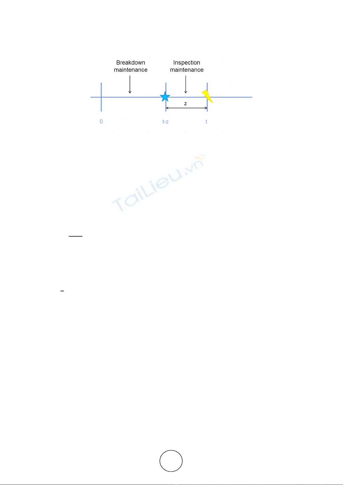
Figure 1 Breakdown and Inspection Maintenance
As can be seen from figure 1, a fault arising within a time period (0,t) is associated with a
delay time z, the probability of occurrence of the event being ∆. is the probability
density function of the delay time z. A fault arising within the time duration (0, t-z) will undergo
a breakdown maintenance whereas a fault arising within the time duration (t-z, t) will undergo
an inspection maintenance.
Summing up all possible values of z, the probability of a breakdown defect occurring, b(t)
can be expressed as follows;
Eqn 1
Assuming that the inspections are carried out at fixed intervals of t hours and the duration
of each inspection is constant. That implies;
Eqn 2
1
It is to be noted here that the probability of a breakdown defect occurring is independent of
the arrival rate of the defect per unit time but dependant on the delay time. The delay time can
be estimated only when a fault has occurred and it has led to a breakdown failure. Hence if a
breakdown failure can exist when a fault has arisen, then it can be said that the probability of
the failure being a breakdown failure, b (t) is a conditional probability (excluding the case of a
sudden failure without any delay time).
2.1. Assumptions made in downtime model formation
• A fault arising within (0,t) has a delay time z
• Probability of occurrence of this event is f(z)dz
• f(z) is the pdf of z
• Inspections are carried out at fixed intervals of t hours.
• The duration of each inspection is constant.
• System downtime during inspection is j hours
• Downtime for carrying out breakdown maintenance is J hours
• Inspection period is of t hours

Rahul Ramachandran, Dr. K. Sunil Kumar and Roy V. Paul
http://www.iaeme.com/IJM/index.as 19 editor@iaeme.com
• Q is the frequency of arrival of defects
• Machinery faults are assumed to be repaired immediately; J<<t
• A good inspection standard is assumed to be present.
• All defects are assumed to be detected.
• An identified defect is assumed to be repaired and the system put back into service within the
inspection period.
• The delay time, z is independent of its time of origin.
• Faults are assumed to be originated at uniform time intervals over the time between inspections.
As a consequence of the above assumptions, the expected downtime per unit time, D(t) can
be expressed as follows;
Eqn 3
{
+ ! " ∗
∗ " $ ∗ $ }
/ ! "+
That implies,
Eqn 4
[(+)∗∗*
+( ]
Substituting value for b(t) obtained from Eqn. 2 in Eqn. 4;
Eqn 5
[(+)∗∗{
,
-}*
+( ]
During literature survey, it came to light that the probability density function was more
close to following a Weibull distribution or a Normal distribution. Similar studies carried out
in the field of maintenance and reliability had used either a Weibull distribution or a Normal
distribution. Due to the simplicity associated with the Normal distribution, the probability
density function of the delay time is assumed to follow a Normal distribution.
That implies;
Eqn 6
1
√201
2
345
6766
Where 8 is the mean of the delay time and 9
:
stands for the standard deviation of the delay
time. The delay time associated with a failure is normally a positive value. Also in cases where
a sudden failure occurs as soon as a fault develops the value of delay time will be zero. It is to
be noted that the delay time is never a negative value due to the fact that a fault could be
followed by a failure but a failure is never followed by a fault.

Maintenance Modelling of Shipboard Machinery by Delay Time Analysis
http://www.iaeme.com/IJM/index.as 20 editor@iaeme.com
That implies;
Eqn 7
≥0
From Eqn. 7 it is very evident that there exists a positive chance for the observation depicted
in Eqn6 being a negative value. This is not considered to be a favourable observation. Hence it
is assumed that the probability density function of delay time follows a truncated standard
normal distribution, truncated at 0 with mean of the delay times, 80 and standard deviation
of the delay time, 9
:
1
Thus the probability density function of delay time is as follows;
Eqn 8
2
√20
2
3
66
Substituting the value of probability density function obtained from Eqn. 8 into the equation
for the expected down time per unit time, Eqn. 5;
That implies;
Eqn 9
[(+)∗∗{
,
-
:
√:=
436
6
}*
+( ]
Eqn. 9 depicts the estimated down time per unit time of the equipment. This is the final
form of the down time model that we have formulated.
2.2. Model Validation
As an example, the maintenance requirements of fuel valves used in Wartsila A6L20C are
considered. It should be noted here that the following information was gathered from logged
historical records, real time operating data and are complimented by expert judgements where
data was not readily available.
The down time due to inspection, j = 30 minutes = 0.5 hours
Down time for breakdown maintenance, J = 12 hours
Arrival rate of defects, Q = 0.00048 per hour
From Eqn. 9,
[(+)∗∗{
,
-
:
√:=
436
6
}*
+( ]
Substituting the values of j, J and Q into Eqn9,
Eqn. 10,
[0.5+0.00048∗∗{
,
-B
:
√:=
436
6
C∗12
+0.5 ]


![Tài liệu học tập Hệ thống điều khiển điện - khí nén và thủy lực [mới nhất]](https://cdn.tailieu.vn/images/document/thumbnail/2021/20211005/conbongungoc09/135x160/811633401135.jpg)
![Tính chọn lắp ghép tiêu chuẩn giữa áo trục và trục chân vịt tàu thủy [chuẩn nhất]](https://cdn.tailieu.vn/images/document/thumbnail/2021/20210219/caygaocaolon10/135x160/5291613732560.jpg)


![Bài giảng Vi điều khiển Nguyễn Huy Hoàng: Tổng hợp kiến thức [Chuẩn nhất]](https://cdn.tailieu.vn/images/document/thumbnail/2026/20260316/hoatrami2026/135x160/72211773806757.jpg)


![Bài giảng Tự động hoá thiết bị điện [chuẩn nhất]](https://cdn.tailieu.vn/images/document/thumbnail/2026/20260312/hoabattu2026/135x160/61691773631881.jpg)
