Lecture Monte carlo simulations: Application to lattice models: Part II

VSOP19, Quy Nhon 3-18/08/2013

Ngo Van Thanh, Institute of Physics, Hanoi, Vietnam.

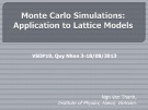
Part II. Monte Carlo Simulation Methods

II.1. The spin models II.2. Boundary conditions II.3. Simple sampling Monte Carlo methods II.4. Importance sampling Monte Carlo methods

A Guide to Monte Carlo Simulations in Statistical Physics

Monte Carlo Simulation in Statistical Physics: An Introduction

D. Landau and K. Binder, (Cambridge University Press, 2009).

Understanding Molecular Simulation : From Algorithms to Applications

K. Binder and D. W. Heermann (Springer-Verlag Berlin Heidelberg, 2010).

Frustrated Spin Systems

D. Frenkel, (Academic Press, 2002).



Lecture notes PDF files : http://iop.vast.ac.vn/~nvthanh/cours/vsop/ Example code : http://iop.vast.ac.vn/~nvthanh/cours/vsop/code/

H. T. Diep, 2nd Ed. (World Scientific, 2013).

II.1. The spin models



Introduction Spin model = spin kind + lattice structure (with including the dimension)



Spin kinds :

Ising



Lattice structure :

Heisenberg

Simple cubic (SC)

Body center cubic (BCC)

Face center cubic (FCC)

Stacked triangular (hexagonal)



…

Dimensions : 2D, 3D or films



n-vector model The hamiltonian

(2.1)

n : number of conponent

n = 0 : The Self-Avoiding Walks n = 1 : Ising model n = 2 : XY model n = 3 : Heisenberg model



exchange interaction J



: Ferromagnetic interaction : Antiferromagnetic interaction : Spin glass

The sum is taken over

nearest neighbours spin pair

next nearest neighbours spin pair …



Ising spin model The hamiltonian



the probability that the system is in state s

(2.2)



For the ferromagnetic Ising model on 2D simple cubic lattice



(2.3)

The energy

(2.4)

XY spin model





The hamiltonian

This is the special case of the n-vector model, for n = 2

 Using polar coordinate, with and

(2.5)

the system in a external magnetic field



(2.6)

(2.7)

Heisenberg spin model





The hamiltonian with

This is the special case of the n-vector model, for n = 3



The equation of motion in the continuum limit

(2.8)



(2.9)

The Potts model The standard Potts model, spin

: is the Kronecker delta

(2.10)

(2.11)

II.2. Boundary conditions

Periodic boundary condition (PBC)

Free boundary condition  Using for a thin-film geometry



s s e n k c h t

l i f

Applying the free boundary condition on z-direction only Use PBC on (x, y) plane

II.3. Simple sampling Monte Carlo methods



Comparisons of methods for numerical integration of given functions:

Simple methods Consider a definite integral



(2.12)



y y0



f(x)

draw a box extending from a to b and from 0 to y0 Using random numbers drawn from a uniform distribution drop N points randomly into the box count the number N0 which fall below f(x) An estimate for the integral

(2.13)

x a b

 Crude method



choose N values of x randomly, then calculate f(x)



(2.14)

Intelligent methods : control variate method

(2.15)



where

selects a integrable function



Simulation of radioactive decay : Consider sample of N nuclei which decay at rate



(2.16)



the rate of decay

(2.17)

the nuclei is chosen randomly The number of undecayed nuclei



Simulation



Dividing the time into discrete intervals



N0 : the initial number of nuclei,  related to the ‘half-life’ of the system



during the time interval, test for decay of each undecayed nucleus



Determine the number of undecayed nuclei

Increasing the time step, then repeat the process



Program structure N = N0 ; NP = N0

LOOP from 1 to NP ! Loop over each remaining parent nucleus

LOOP from (t = dt) to Tmax , step dt

R = uniform_RandomNumber()

! 0  R  1

IF ( R < λ dt ) THEN

N = N-1

END IF

END LOOP over nuclei

NP = N

Record t, N

END LOOP over time

Source : radioactive_decay.f90

PROGRAM RADIOACTIVE_DECAY IMPLICIT NONE REAL :: t,tmax,dt,r,lambda INTEGER :: n,n0,np,nt,i ! CALL RANDOM_SEED() n0 = 1000; tmax = 50.0 dt = 0.1; lambda = 0.1 n = n0; t = 0.0 DO WHILE (t <= tmax .AND. n > 0) t = t + dt np = n DO i = 1,np CALL RANDOM_NUMBER(r) IF (r < lambda*dt) n = n - 1 END DO nt = NINT(n0*exp(-t*lambda)) print*,t,n,nt END DO END PROGRAM RADIOACTIVE_DECAY



Finding the groundstate of a hamiltonian Consider a system of Ising spins



Algorithm



Randomly chosen an initial state of the system Choose a random site on the lattice Try to overturn the spin, determining the change in energy if the energy is lowered, then accept the overturn of the spin otherwise it is left unchanged, go to the next site.

 We can use different initial configurations, one tests to see

the system is then either in the groundstate or in some metastable state.

if the same state is reached as before if a lower energy state is found.

Source : groundstate.f90

PROGRAM GROUNDSTATE IMPLICIT NONE INTEGER, PARAMETER :: N = 10 REAL,DIMENSION(n,n) :: S INTEGER :: i,j,k,l,ip,im,jp,jm REAL :: r,e1,e2,temp ! initial configuration CALL RANDOM_SEED() CALL RANDOM_NUMBER(S) DO i = 1,n DO j = 1,n IF (S(i,j) > 0.5) THEN S(i,j) = 1.0 ELSE S(i,j) = -1.0 ENDIF ENDDO ENDDO print*,0,etot()

DO l = 1,60 ! Simulation DO k = 1,40 CALL RANDOM_NUMBER(r) i = INT(r*float(n))+1 CALL RANDOM_NUMBER(r) j = INT(r*float(n))+1 ! periodic boundary condition ip = i + 1; im = i - 1 jp = j + 1; jm = j - 1 IF (ip > n) ip = 1; IF (im < 1) im = n IF (jp > n) jp = 1; IF (jm < 1) jm = n ! calculate the energy e1 = -S(i,j)*(S(ip,j)+S(im,j)+S(i,jp)+S(i,jm)) e2 = -e1 IF (e2 <= e1) S(i,j) = -S(i,j) ENDDO print*,l,etot() ENDDO

CONTAINS ! list of subroutine/function REAL FUNCTION etot temp = 0.0 DO i = 1,n ip = i + 1; im = i - 1 IF (ip > n) ip = 1 IF (im < 1) im = n DO j = 1,n jp = j + 1; jm = j - 1 IF (jp > n) jp = 1 IF (jm < 1) jm = n temp = temp & - S(i,j)*(S(ip,j)+S(im,j)+S(i,jp)+S(i,jm)) ENDDO ENDDO etot = 0.5*temp/float(n*n) END FUNCTION etot ! END PROGRAM GROUNDSTATE



Generation of random walks Introduction

path formed by randomly adding new bonds to the end of the existing walk



A random walk consists of a connected

The mean-square end-to-end distance

(2.18)

: critical exponent

: non-universal constants



The partition function

: correction to scaling exponent

(2.19)

: an effective coordination number

 Random walks (RW)



used for the description of diffusion phenomena

the end-to-end distance



(2.20)

Simulation of the simple random walk

Picking a starting point

Generating a random number to determine the direction of each subsequent

Calculating the end-to-end distance

 non-reversal random walk (RNNW)

Performing a statistical analysis of the resultant distribution

The choice of the (n + 1) step from the nth step of a return to the point reached at the (n - 1) step is forbidden

! number-of-samples ! initial position ! number of step



id = INT(r*4.0) SELECT CASE(id) CASE (0)  x = x + 1 CASE (1)  x = x - 1 CASE (2)  y = y + 1 CASE (3)  y = y - 1 END SELECT

Algorithm of random walks DO i = 1 to ns x = 0; y = 0 DO j = 1 to N ENDDO accumulate-results ENDDO

the end-to-end distance

Source : randomwalk.f90

INTEGER, PARAMETER :: ns = 1000,n = 100 INTEGER :: i,j,x,y,id REAL :: r,d,d2,temp CALL RANDOM_SEED() d = 0.0; d2 = 0.0 DO i=1,ns x = 0; y = 0 DO j = 1,n CALL RANDOM_NUMBER(r) id = INT(r4.0) SELECT CASE (id) CASE (0) x = x + 1 CASE (1) x = x - 1 CASE (2) y = y + 1 CASE (3) y = y - 1 END SELECT ENDDO temp = float(x2+y2) d = d + sqrt(temp); d2 = d2 + temp ENDDO d = d/float(ns); d2 = d2/float(ns) print,ns,n,d,d2

Algorithm of non-reversal random walks



! number-of-samples DO i = 1 to ns

x = 0; y = 0 ! initial position

xp = 0; yp = 0 ! previous position

! number of step DO j = 1 to N

repeat

xt = x; yt = y ! template position

generate-one-step (x; y)

until ((x  xp) or (y  yp))

xp = xt

yp = yt

ENDDO

accumulate-results

ENDDO

Source : nr_randomwalk.f90

PROGRAM NR_RANDOM_WALKS IMPLICIT NONE INTEGER, PARAMETER :: ns = 1000,n = 100 INTEGER :: i,j,x,y,id,xp,yp,xt,yt REAL :: r,d,d2,temp LOGICAL :: test ! CALL RANDOM_SEED() d = 0.0; d2 = 0.0 CALL NRRW() ! non-reversal random walks d = d/float(ns); d2 = d2/float(ns) print*,ns,n,d,d2 CONTAINS SUBROUTINE NRRW … END SUBROUTINE NRRW END PROGRAM NR_RANDOM_WALKS

SUBROUTINE NRRW DO i=1,ns x = 0; y = 0; xp = x; yp = y DO j = 1,N xt = x; yt = y; test = .FALSE. DO WHILE(.NOT.test) CALL RANDOM_NUMBER(r) id = INT(r*4.0) IF (id == 0) THEN x = xt + 1; y = yt ELSEIF (id == 1) THEN x = xt - 1; y = yt ELSEIF (id == 2) THEN y = yt + 1; x = xt ELSEIF (id == 3) THEN y = yt - 1; x = xt ENDIF IF ((x .NE. xp).OR.(y .NE.yp)) test =.TRUE. ENDDO xp = xt; yp = yt ENDDO temp = float(x**2+y**2) d = d + sqrt(temp); d2 = d2 + temp ENDDO END SUBROUTINE NRRW

 Self-avoiding walks (SAW)



Used to probe the configurations of flexible

The walker dies when attempting to intersect

macromolecules in the solvents



a portion of the already completed walk

Picking a starting point

Simulations

Generating a random number to the different possible choices for the next step

If the new site is one which already contains a portion of the walk, then the process is terminated at the Nth step.

effective exponent



(2.21)

For , the effective exponent is then related to the true value

(2.22)

the current estimates for

(2.23)



 The exponent

K. Kremer and K. Binder, Comput. Phys. Rep. 7, 261 (1988)

Using the equation (2.19), we have

(2.24)

 using ‘symmetric’ values in step number

(2.25)



Algorithm of Self-avoiding walks integer lattice(-N:N;-N:N); do sample = 1 to n-of-samples step = 0; x = 0; y = 0; xc = 0; yc = 0; repeat repeat generate-one-step(xnew, ynew); until lattice(xnew, ynew)  sample + 1; if lattice(xnew, ynew) = sample then terminate = true else lattice(x, y) = sample; x = xc; y = yc; lattice(x, y) = sample + 1; xc = xnew; yc = ynew; step = step + 1; endif until (terminate or step = N); accumulate-results enddo

Source: sa_walk.f90

…

PROGRAM SELF_AVOIDING_WALKS IMPLICIT NONE INTEGER, PARAMETER :: ns = 100,n = 100 INTEGER, DIMENSION(-n:n,-n:n) :: lattice INTEGER :: i,x,y,xt,yt,id,step,nn REAL :: r,d,d2,temp LOGICAL :: terminate,newsite ! CALL RANDOM_SEED() d = 0.0; d2 = 0.0 CALL SAW() ! self avoiding walks d = d/float(ns); d2 = d2/float(ns) print*,ns,n,d,d2 ! CONTAINS SUBROUTINE SAW END SUBROUTINE SAW ! END PROGRAM SELF_AVOIDING_WALKS

SUBROUTINE SAW DO i = 1,ns lattice = 0 x = 0; y = 0 step = 0; terminate = .FALSE. DO WHILE ((.NOT. terminate) .AND. (step <= n)) xt = x; yt = y nn = lattice(x+1,y) + lattice(x-1,y) & + lattice(x,y+1) + lattice(x,y-1) IF (nn == 4) THEN terminate = .TRUE. ELSE newsite = .FALSE. DO WHILE (.NOT. newsite) CALL RANDOM_NUMBER(r) id = INT(r*4.0)

IF (id == 0) THEN x = xt + 1; y = yt ELSEIF (id == 1) THEN x = xt - 1; y = yt ELSEIF (id == 2) THEN y = yt + 1; x = xt ELSEIF (id == 3) THEN y = yt - 1; x = xt ENDIF IF (lattice(x,y) == 0) newsite = .TRUE. ENDDO step = step + 1 lattice(x,y) = 1 ENDIF ENDDO temp = float(x**2+y**2) d = d + sqrt(temp) d2 = d2 + temp ENDDO END SUBROUTINE SAW

Thermal Averages by the Simple Sampling Method

 The model

Consider a polymer chain,



: attractive energy between two nearest neighbor monomers

 Defination



(2.26)

The distribution

number of SAW configurations of N steps with n nearest-neighbor contacts

(2.27)

number of SAW configurations of N steps with n nearest-neighbor contacts and an end-to-end vector .

 The averages of interest

(2.28)

 The specific heat C per bond of the chain

(2.29)

 Using Eq. (2.28), we have

(2.30)

(2.31)

II.4. Importance sampling Monte Carlo methods

Introduction



Consider a spin model, the Hamiltonian is given by

used for the study of phase transitions at finite temperature



(2.32)

(2.33)



the averages

the thermal average of any observable

(2.34)



probability density



(2.35)

integrates Eq. (2.34) over all states with their proper weights

 We consider a process where the phase space points are selected

according to some probability

(2.36)



(2.37)



A natural choice for

simple average

(2.38)

Algorithm (Metropolis method)

The configurations are generated from a previous state using a transition probability which depends on the energy difference between the initial and final states

The master equation of probability of the system



that is in the state n at time t

(2.39)



: is the transition rate for In the equilibrium process, the condition of detailed balance:

 We have

(2.40)

The probability of the nth state occurring in a classical system



(2.41)

If we produce the nth state from the mth state



From Eqs. (2.40) and (2.41), we have



(2.42)

The choice of rate (Metropolis form)

(2.43)

: is the time required to attempt a spin-flip

 Metropolis importance sampling Monte Carlo scheme

Ising model

(1) Choose an initial state

(2) Choose a site i

(3) Calculate the energy change E which results if

the spin at site i is overturned

(4) Generate a random number r such that 0 < r < 1

(5) If exp(-E/kBT) > r, flip the spin

(6) Go to the next site and go to (3)



 Program structure

initialize the lattice

SUBROUTINE equilibrating ! Equilibrating process DO ieq = 1 to N_eq CALL monte_carlo_step() ENDDO END SUBROUTINE ! Averaging process SUBROUTINE averaging DO iav = 1 to N_av CALL monte_carlo_step() do-analysis ENDDO END SUBROUTINE SUBROUTINE monte_carlo_step generate-one-sweep END SUBROUTINE

Source : ising_2dsl.f90

 Fortran code (ferromagnetic Ising spin model on 2D square lattice)

PROGRAM ISING_2D_SL IMPLICIT NONE INTEGER, PARAMETER :: n = 10,nms = n*n,nt = 20 REAL,DIMENSION(n,n) :: S INTEGER :: i,j,ip,im,jp,jm,ie,ia,ms,it,neq,nav REAL :: r,tmin,tmax,t,dt,e1,e2,temp REAL :: ener,magn ! CALL RANDOM_SEED() neq = 2000 nav = 4000 tmin = 0.5; tmax = 4.0

! initial configuration ! equilibrating process

! averaging process

! list of subroutines/functions

dt = (tmax-tmin)/float(nt-1) t = tmin ! DO it = 1,nt CALL spin_conf() CALL equilibrating() ener = 0.0 magn = 0.0 CALL averaging() ener = ener/float(nav) magn = magn/float(nav) print*, t,ener,magn t = t + dt ENDDO

CONTAINS … END PROGRAM ISING_2D_SL

! list of subroutines/functions

CONTAINS ! SUBROUTINE spin_conf CALL RANDOM_NUMBER(S) DO i = 1,n DO j = 1,n IF (S(i,j) > 0.5) THEN S(i,j) = 1.0 ELSE S(i,j) = -1.0 ENDIF ENDDO ENDDO END SUBROUTINE spin_conf ! SUBROUTINE equilibrating DO ie = 1, neq CALL monte_carlo_step() ENDDO END SUBROUTINE equilibrating

! Calculate the average energy per spin

SUBROUTINE averaging DO ia = 1, nav CALL monte_carlo_step() temp = 0.0 DO i = 1,n ip = i + 1; im = i - 1 IF (ip > n) ip = 1 IF (im < 1) im = n DO j = 1,n jp = j + 1; jm = j - 1 IF (jp > n) jp = 1 IF (jm < 1) jm = n temp = temp -S(i,j)*& (S(ip,j)+S(im,j)+S(i,jp)+S(i,jm)) ENDDO ENDDO ener = ener + 0.5*temp/float(n*n)

! Calculate the average magnetization per spin

temp = 0.0 DO i = 1,n DO j = 1,n temp = temp + S(i,j) ENDDO ENDDO magn = magn + abs(temp)/float(n*n) ENDDO END SUBROUTINE averaging

! periodic boundary condition

! calculate the different energy

SUBROUTINE monte_carlo_step DO ms = 1,nms ! number of Monte Carlo step CALL RANDOM_NUMBER(r) i = INT(r*float(n))+1 CALL RANDOM_NUMBER(r) j = INT(r*float(n))+1 ip = i + 1; im = i - 1 jp = j + 1; jm = j - 1 IF (ip > n) ip = 1 IF (im < 1) im = n IF (jp > n) jp = 1 IF (jm < 1) jm = n e1 = -S(i,j)*(S(ip,j)+S(im,j)+S(i,jp)+S(i,jm)) e2 = -e1 CALL RANDOM_NUMBER(r) IF (r < exp(-(e2-e1)/t)) S(i,j) = -S(i,j) ENDDO END SUBROUTINE monte_carlo_step



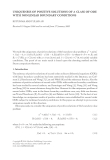
Ferromagnetic Ising spin model on square lattice

Energy vs temperature for N = 10



Ferromagnetic Ising spin model on square lattice

Magnetization vs temperature for N = 10

Exercises

 modify the program «ising_2dsl.f90» :



Adding the calculations for specific heat and susceptibility

ener2 = ener2 + (0.5*temp/float(n*n))**2 magn2 = magn2 + (temp/float(n*n))**2



cv = float(n*n)*(ener2 – ener*ener)/t/t chi = float(n*n)*(magn2 – magn*magn)/t

For the case of three dimensions simple cubic lattice

Local energy :

e1 = -S(i,j,k)*(S(ip,j,k)+S(im,j,k)+S(i,jp,k)+S(i,jm,k) +S(i,j,kp)+S(i,j,km))



Ferromagnetic Ising spin model on square lattice

Specific heat vs temperature for N = 10



Ferromagnetic Ising spin model on square lattice

Magnetic susceptibility vs temperature for N = 10



Ferromagnetic Ising spin model on simple cubic lattice

Energy, magnetization, specific heat and susceptibility vs temperature for N = 12

 Write a new program for ferromagnetic XY spin model on square

lattice

Including the calculations for specific heat and susceptibility



The local energy

e1 = -SX(i,j)*(SX(ip,j)+SX(im,j)+SX(i,jp)+SX(i,jm)) -SY(i,j)*(SY(ip,j)+SY(im,j)+SY(i,jp)+SY(i,jm))

Generate a new XY spin with random orientation

! orientation

CALL RANDOM_NUMBER(r)

PHI = 2.0*3.14159260*r SXN = COS(PHI) SYN = SIN(PHI)

Source : xy_2dsl.f90

 Fortran code (ferromagnetic XY spin model on square lattice)

IMPLICIT NONE

PROGRAM XY_2D_SL

REAL,PARAMETER:: pi2 = 2.0*3.1415926

INTEGER, PARAMETER :: n = 10,nms = n*n,nt = 20

INTEGER :: i,j,ip,im,jp,jm,ie,ia,ms,it,neq,nav

REAL,DIMENSION(n,n) :: sx,sy

REAL :: r,tmin,tmax,t,dt,e1,e2,si,phi,sxn,syn,temp

REAL :: sxt,syt,ener,magn

CALL RANDOM_SEED()

neq = 20000

nav = 40000

tmin = 0.1; tmax = 2.0

dt = (tmax-tmin)/float(nt-1) t = tmin ! DO it = 1,nt

! initial configuration

CALL spin_conf() CALL equilibrating() ener = 0.0; magn = 0.0 CALL averaging() ener = ener/float(nav) magn = magn/float(nav) print*, t,ener,magn t = t + dt ENDDO

! list of subroutines/functions

CONTAINS

SUBROUTINE spin_conf ! DO i = 1,n DO j = 1,n CALL RANDOM_NUMBER(r) phi = pi2*r sx(i,j)=cos(phi) sy(i,j)=sin(phi) ENDDO ENDDO END SUBROUTINE spin_conf ! SUBROUTINE equilibrating DO ie = 1, neq CALL monte_carlo_step() ENDDO END SUBROUTINE equilibrating

+ sx(i,jp) + sx(i,jm)) &

+ sy(i,jp) + sy(i,jm))

SUBROUTINE averaging DO ia = 1, nav CALL monte_carlo_step() temp = 0.0 DO i = 1,n ip = i + 1; im = i - 1 IF (ip > n) ip = 1 IF (im < 1) im = n DO j = 1,n jp = j + 1; jm = j - 1 IF (jp > n) jp = 1 IF (jm < 1) jm = n temp = temp - sx(i,j)*(sx(ip,j) + sx(im,j) & - sy(i,j)*(sy(ip,j) + sy(im,j) & ENDDO ENDDO

ener = ener + 0.5*temp/float(n*n) sxt = 0.0; syt = 0.0 DO i = 1,n DO j = 1,n sxt = sxt + sx(i,j) syt = syt + sy(i,j) ENDDO ENDDO magn = magn + sqrt(sxt**2 + syt**2)/float(n*n) ENDDO END SUBROUTINE averaging

! periodic boundary condition

SUBROUTINE monte_carlo_step DO ms = 1,NMS CALL RANDOM_NUMBER(r) i = INT(r*float(n))+1 CALL RANDOM_NUMBER(r) j = INT(r*float(n))+1 ip = i + 1; im = i - 1 jp = j + 1; jm = j - 1 IF (ip > n) ip = 1 IF (im < 1) im = n IF (jp > n) jp = 1 IF (jm < 1) jm = n

! calculate the local energy

sxt = sx(ip,j)+sx(im,j)+sx(i,jp)+sx(i,jm) syt = sy(ip,j)+sy(im,j)+sy(i,jp)+sy(i,jm) e1 = -sx(i,j)*sxt - sy(i,j)*syt CALL RANDOM_NUMBER(r) phi = pi2*r sxn=cos(phi) syn=sin(phi) e2 = -sxn*sxt -syn*syt CALL RANDOM_NUMBER(r) IF (r < exp(-(e2-e1)/t)) THEN sx(i,j) = sxn sy(i,j) = syn ENDIF ENDDO END SUBROUTINE monte_carlo_step ! END PROGRAM XY_2D_SL



Ferromagnetic XY spin model on square lattice



Energy and magnetization vs temperature for N = 10

There exist two phases

A low-temperature-phase with a quasi-long range order, where most spins are aligned and the correlation-function decays with a power law An unordered high-temperature-phase where the correlation-function decays exponentially



The phase transition is called «Kosterlitz-Thouless transition»

Counterclockwise vortices

 Write a new program for ferromagnetic Heisenberg spin model on two

dimensions square lattice

The local energy

e1 = -SX(i,j)*(SX(ip,j)+SX(im,j)+SX(i,jp)+SX(i,jm)) -SY(i,j)*(SY(ip,j)+SY(im,j)+SY(i,jp)+SY(i,jm)) -SZ(i,j)*(SZ(ip,j)+SZ(im,j)+SZ(i,jp)+SZ(i,jm))

Generate a new Heisenberg spin with random module and orientation

! orientation

CALL RANDOM_NUMBER(r)

! projection of SZ

PHI = 2.0*3.14159260*r CALL RANDOM_NUMBER(r)

SZN = 2.0*r-1.0 SI = SQRT(1-SZN*SZN) SXN = SI*COS(PHI) SYN = SI*SIN(PHI)

For two dimensions triangular lattice

The local energy

e1 = -S(i,j)*(S(ip,j)+S(im,j)+S(i,jp)+S(i,jm) + S(ip,jm)+S(im,jp))

For 3D stracked triangular lattice

e1 = -S(i,j,k)*(S(ip,j,k)+S(im,j,k)+S(i,jp,k)+S(i,jm,k) +S(ip,jm,k)+S(im,jp,k) +S(i,j,kp) +S(i,j,km))

Source : ising_2dtl.f90

 Fortran code (ferromagnetic Ising spin model on triangular lattice)

IMPLICIT NONE

PROGRAM ISING_2D_TL

INTEGER, PARAMETER :: n = 10,nms = n*n,nt = 40

REAL,DIMENSION(n,n) :: S

REAL :: r,tmin,tmax,t,dt,e1,e2,temp

INTEGER :: i,j,ip,im,jp,jm,ie,ia,ms,it,neq,nav

REAL :: ener,magn

CALL RANDOM_SEED()

neq = 20000

nav = 40000

tmin = 1.0; tmax = 6.0

dt = (tmax-tmin)/float(nt-1) t = tmin ! DO it = 1,nt CALL spin_conf() ! initial configuration CALL equilibrating() ener = 0.0; magn = 0.0 CALL averaging() ener = ener/float(nav) magn = magn/float(nav) print*, t,ener,magn t = t + dt ENDDO CONTAINS ! list of subroutine/function

SUBROUTINE spin_conf ! CALL RANDOM_NUMBER(S) DO i = 1,n DO j = 1,n IF (S(i,j) > 0.5) THEN S(i,j) = 1.0 ELSE S(i,j) = -1.0 ENDIF ENDDO ENDDO END SUBROUTINE spin_conf ! SUBROUTINE equilibrating DO ie = 1, neq CALL monte_carlo_step() ENDDO END SUBROUTINE equilibrating

SUBROUTINE averaging DO ia = 1, nav CALL monte_carlo_step() temp = 0.0 DO i = 1,n ip = i + 1; im = i - 1 IF (ip > n) ip = 1 IF (im < 1) im = n DO j = 1,n jp = j + 1; jm = j - 1 IF (jp > n) jp = 1 IF (jm < 1) jm = n temp = temp - S(i,j)*(S(ip,j)+S(im,j) & +S(i,jp)+S(i,jm) + S(ip,jm)+S(im,jp) ) ENDDO ENDDO ener = ener + 0.5*temp/float(n*n)

temp = 0.0 DO i = 1,n DO j = 1,n temp = temp + S(i,j) ENDDO ENDDO magn = magn + abs(temp)/float(n*n) ENDDO END SUBROUTINE averaging

! calculate the energy

+ S(ip,jm)+S(im,jp) )

SUBROUTINE monte_carlo_step DO ms = 1,NMS CALL RANDOM_NUMBER(r); i = INT(r*float(n))+1 CALL RANDOM_NUMBER(r); j = INT(r*float(n))+1 ! periodic boundary condition ip = i + 1; im = i - 1 jp = j + 1; jm = j - 1 IF (ip > n) ip = 1 IF (im < 1) im = n IF (jp > n) jp = 1 IF (jm < 1) jm = n e1 = -S(i,j)*(S(ip,j)+S(im,j)+S(i,jp)+S(i,jm) & e2 = -e1 CALL RANDOM_NUMBER(r) IF (r < exp(-(e2-e1)/t)) S(i,j) = -S(i,j) ENDDO END SUBROUTINE monte_carlo_step END PROGRAM ISING_2D_TL



Ferromagnetic Ising spin model on 2D triangular lattice

Energy vs temperature for N = 10



Ferromagnetic Ising spin model on 2D triangular lattice

Magnetization vs temperature for N = 10

Lecture Monte carlo simulations: Application to lattice models: Part II - TS. Ngô Văn Thanh